MagIC Help Library |
|||
|
|
|
||
MagIC Help Library |
|||
|
|
|
||
1 Introduction
1.1 Preface
The Magnetics Information Consortium (MagIC) initiative has been established to address the need for a public digital archive for the international magnetics research community. As a multi-user facility MagIC provides a place for the community to archive new data as soon after their collection as reasonable, preferably at the time of publication in the peer-reviewed literature. These data are stored in and served from an Oracle 10x database that is part of the overarching online EarthRef.org database, while software tools are provided to help the scientist in preparing data for automated uploading. The MagIC Databases Team already has transferred the data and metadata of existing magnetic databases (GPMDB, PINT, etc.) created under the auspices of IAGA into the MagIC database.
The databases of the Magnetics Information Consortium (MagIC) thus contain user-contributed data associated with paleomagnetic and rock magnetic sources. Data may be part of data published in Earth sciences journals, theses or books. These data are contributed on a Publication-by-Publication basis and in the form of two corresponding MagIC Format ASCII Text (*.txt) and Microsoft Excel© SmartBook (*.xls) files created by the MagIC Console Software. These SmartBook files are uploaded into the MagIC database by using the MagIC Contribution Wizard.
1.1.1 Goals and Philosophy
The overarching goal of the Magnetics Information Consortium (MagIC) is to develop and maintain databases and associated information technology for the international paleomagnetic, geomagnetic and rock magnetic community. MagIC is hosted under the umbrella of EarthRef.org allowing coordination with other information technology initiatives in the Earth sciences, such as GERM, SBN and ERESE. This facilitates interdisciplinary research, by allowing ready access to relevant information in related disciplines. MagIC serves the larger scientific and educational community by making its databases freely accessible and by providing visualization tools designed for users with various levels of expertise.
The PMAG Portal and the RMAG Portal (still under development) form the access points to a new generation of community-based paleomagnetic and rock magnetic databases. These web portals share the same underlying MagIC Data Model, allowing for searches and access to information in both databases. Users can upload their own data (for free) using the standard MagIC Metadata and Data Model available online as long as these uploads are associated with a citable publication and the user have registered. Substantial effort has gone into making the data model flexible enough to accommodate the broad range of data collected in rock and paleomagnetic studies. Where feasible, contributors are encouraged to upload all their measurements and descriptions of lab procedures, in addition to their higher level (published) results. Digital information that does not fit readily into the MagIC always can be uploaded and archived in the ERDA online archive.
MagIC is managed with the help of in particular a Steering Committee and a Metadata and Method Codes Committee that both have a wide representation from the paleomagnetic and rock magnetic research community, nationally and internationally. MagIC also promotes a community dialog on how modern paleo, rock and geomagnetic databases should evolve, and what online tools are needed for data analysis. The dialog includes sponsoring discussions at workshops and promoting special sessions at scientific meetings. MagIC has evolved substantially since its inception at the PMAG Workshop held in March 2002 at Scripps Institution of Oceanography in La Jolla.
From the start MagIC has been incorporating PMAG data from the IAGA databases, namely GPMDB, PINT2003, TRANS, PSVRL and SECVR. However, the new data model allows contributors to archive more information than before, and provides ready access to the data online without the need to resort to commercial database software. RMAG is the first attempt to generate a database of rock magnetic data.
1.1.2 User and Data Policy
All data in the MagIC database are User-Contributed and uploaded on a Publication-by-Publication basis. The MagIC database primarily contains Activated Contributions from Peer-Reviewed Publications and Student Theses, including those In Press. These uploads are available to the entire MagIC userbase and are permanently archived under a strict version control. The various user actions, contribution types, levels of data ownership and data deletions are explained in detail below.
All database contributors and users are to adhere to the EarthRef.org Copyright Policy.
Data sets for publications In Preparation or In Review can be uploaded as Private Contributions Only and can be accessed by the data owners alone. These Private Contributions optionally can be set up by the data owner to have Group Access allowing select groups of users to access such hidden MagIC data sets with a group name and password.
Unpublished Data Sets that cannot be published (elsewhere) in the peer-reviewed literature can be uploaded into the MagIC database as an EarthRef.org Data Publication. These uploads should be accompanied with a list of authors, affiliations, a title, a short abstract and a technical note that describes the analytical methods applied. These publications will be assigned an EarthRef.org DOI and their citation will be permanently stored in the EarthRef.org Reference Database.
Activated Contributions will undergo Data Reviews by editors and referees representing the international paleo- and rock magnetic research community. These Data Reviews are meant to help improve the quality of the data uploads and are not meant to critique the science and conclusions presented in the publications.
Data owners can manage a contribution to the MagIC database in three different ways:
Once a contribution has been uploaded into the MagIC database, the data owner can restrict its access or provide open access to the world, again in three different ways:
There can only be one data owner per contribution. However, data ownership can change based on the following hierarchy:
Activated Contributions cannot be deleted by the data owners. Private Contributions remain in the database until the data owner replaces it with an activated update or activates an existing private upload. If a private contribution has been Inactive for more than 2 years it will be removed from the data holdings by the MagIC Database Team.
The MagIC Database Team reserves the right to delete any Incorrect or Fraudulent Contributions without any further notice.
Each Activated Contribution will be assigned a Data Editor, who will select at least one Referee to review the data contribution for its correctness, completeness and clarity only. These reviews are meant to help improve the quality of the uploaded data in the MagIC Database. However, these reviews explicitly are not concerned with the science and conclusions presented in the publication.
Once the data review(s) are complete, the data owner should prepare an update of the data contribution and upload this as soon as possible into the MagIC Database. All activated versions of these data contributions will be retained in the database, will receive a time stamp and version number, and can be retroactively included in database searches.
1.1.3 MagIC Database Team and Committee Structure
The MagIC Database Team is responsible for the development and maintenance of the MagIC Database and Website. This team exists of the principal investigators, associated researchers, software engineers and undergraduate students.
The Steering Committee is intended to determine the direction to be followed in the development of paleomagnetic and rock magnetic databases, and includes broad international representation from the overall magnetics community as well as people involved in database development in related fields of Earth sciences.
Metadata and Method Codes Committee
The charge for the Metadata and Method Codes Committee is to engage in continuing broad consultation with the magnetics community on the kinds of information that need to be preserved in magnetic databases, and develop an appropriate metadata template for use in paleomagnetic and rock magnetic databases. In particular, it will be necessary to develop metadata structures that can be effectively exploited for existing lines of research while preserving the flexibility for accessing information required to develop new research ideas. The results of such consultation should then be incorporated into a metadata structure, which will be reviewed by the Steering Committee and presented to researchers in the international community for comment prior to finalizing the database structure. This committee will also be in charge of adding and editing the required method codes and controlled vocabularies.
Editorial and Review Committee
The charge for the MagIC Editors is to oversee the review process of all data submissions into the MagIC Database. They will assign each data contribution to any of the potential reviewers that also may include members outside of this committee.
Geological Timescale Committee
The charge for the Geological Timescale Committee is to work towards a nominal timescale to be used in the MagIC Database and will enhance its search capabilities and helps in the interpretation and compilation of disparate data sets.
The charge for the Paleolocations Committee is to work towards a nominal plate motion model through geological time to be used in the MagIC Database and will enhance its search capabilities and helps in the interpretation and compilation of disparate data sets.
1.1.4 History and Timeline
MagIC evolved from the PMAG Workshop held at Scripps Institution of Oceanography in La Jolla, from 24-26 March 2002. The Abstract Volume for this workshop is available online. At this workshop it was agreed that there is a critical need to update and integrate existing magnetic database efforts sponsored by IAGA to take advantage of the technological advances provided by modern web-based data handling capabilities. In September 2002 a small workshop was held at the Institute for Rock Magnetism at the University of Minnesota to discuss the new design of a new rock magnetic database and its integration with the efforts discussed at PMAG2002. A short report is published in EOS and is available online.
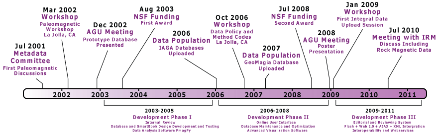
Three development stages mark MagIC's short history. In Phase I we focused on an internal review of the MagIC Data Model, the design of the Oracle 10x Database, the design of the SmartBooks, the coding of the MagIC Console Software and extensive testing. Also the PmagPy data analysis software was developed allowing scientists to translate paleomagnetic measurement data into the MagIC format. In Phase II we started to focus on the design and implementation of the Online Drilldown Interface, to populate, maintain and optimize the MagIC Database, and to implement Advanced Visualizations in the MagIC web portals. Currently we are in Phase III whereby we are planning to implement an Editorial and Reviewing System, we will start to use predominantly Flash, Web 2.0, AJAX and XML in our web and database interfaces, and we will start to work toward full Interoperability with other online databases using Webservices.
1.1.5 Acknowledgements
This Help Library is a public domain document to support the Magnetics Information Consortium (MagIC) in its efforts to promote and facilitate an Information Technology (IT) Infrastructure for the international paleomagnetic, rock magnetic and geomagnetic community. This document came together as a result of discussions between the members of the MagIC Steering Committee and MagIC Metadata Committee formed during the first PMAG Workshop held in La Jolla (USA) in March 2002. It is being updated continuously to make certain that all tools and software can be easily used without too much guidance. To view who is involved in the MagIC consortium, please visit the http://earthref.org/MAGIC/whoswho.htm website.
MagIC is supported by NSF Grants EAR03-18672, EAR07-44107 and EAR07-44108.
1.2 Getting Started
1.2.2 Become a Registered EarthRef.org User
To register click on the Register link in the Topmenu of the EarthRef.org website. If you have forgotten your password or username, please go to the http://earthref.org/databases/ERML/ webpage or click on the Forgot Password link in the Topmenu. Twice a year you will be sent a Reminder Email with all registration info and a simple link to edit your user profile.
Registration is required if you want to upload your data into the MagIC database. In return, you will be informed of new features on the website, software updates and other information related to the MagIC initiative through Bi-monthly Newsletters and other email alerts. Searching and downloading data from the database does not require an user name and password.
1.2.3 Reviewer and Editor Responsibilities
A reviewer of a MagIC database contribution is responsible for comparing the uploaded data to the data in the corresponding paper and commenting on any errors or omissions. An online review system is available to help reviewers with this task.
First the reviewer checks the reference to make sure it is correct and complete. Next the reviewer checks the various tables that have been filled out in the smartbook by the contributor. Tables with location data present the reviewer with a map so they can quickly check if the location is correct. Then the reviewer checks the method codes used by the contributor and verifies that they are correct and not missing significant descriptions of the data. Finally the reviewer writes any additional comments to the contributor and marks the review complete.
An editor for the MagIC database is responsible for overseeing the reviewing of new contributions to the MagIC database. The editor will be able to delegate the review process of new contributions to reviewers or review the contributions themselves. Reviews should be done in a timely manner. About a month to review a contribution is an appropriate timeline.
1.2.4 Online Search Features and Data Uploading
Two separate web portals have been developed within MagIC for Paleomagnetism (PMAG) and Rock Magnetism (RMAG). Both interrogate the same underlying MagIC and EarthRef.org databases. This ensures that the search forms for typical paleomagnetic and rock magnetic searches can be kept simple and transparent. However, it does not prevent paleomagnetists from performing rock magnetic queries when searching within the PMAG Web Portal, and vice versa, when starting out from within the RMAG Web Portal. By design each portal is merely a different entry point into the same database.
To search from within the PMAG Web Portal follow the http://earthref.org/MAGIC/search/ link. Here we provide you with search options of location, data type, geological age and reference. You can also do map searches using the Map filter. Each of these searches give you a simple first page from which you can drill down all the way to the measurement level. An advanced search lets you perform more complex searches, including custom Boolean expressions.
Once the RMAG Web Portal is active, to start the RMAG Web Portal follow the http://earthref.org/databases/RMAG/ link. From this web page you can perform simple searches based on experiment type or condition, sample type and reference. Again, in each search you will be allowed to drill down to the measurement level, and an advanced search option lets you perform more demanding search tasks.
The Online Upload Wizard has been developed to help you upload your own data. Uploading can be started by following the http://earthref.org/MAGIC/upload.htm link. The only requirement here is that you are a Registered EarthRef.org User. Uploading data can typically be completed in less than 5 minutes, depending on the number of data records involved. The Online Upload Wizard will ask you to log-in under your EarthRef.org Username and to upload two files (a Microsoft Excel© file and an plain text version of the same file) that were automatically generated by processing your data with the MagIC Console Software. These two files will be archived in the EarthRef.org database while the data and metadata they contain will be parsed into the MagIC database.
This data uploading naturally complements the scientific process of preparing your data for submittal to any Earth science journal. Because you can upload your data into the MagIC database while keeping it Private (as described in the User and Data Policy) you can use all visualization tools on the MagIC website to study and analyze your data, either on their own right or in combination with data already available in the database. You can also make your data Group Accessible by assigning a group name and password that you personally can give out to your colleagues, co-authors and reviewers. All in all, this approach gives you a multitude of flexibility in working with your paleo and rock magnetic data. When you're ready you can Activate your private contributions and make them Publicly Available to other MagIC and EarthRef.org users.
1.2.5 The MagIC Console Software
Getting your data organized, complete and ready to submit for either a paper publication or ingesting into a database is a time-consuming job. We have developed the MagIC Console Software to aid you in your collation of paleo and rock magnetic data and to make the data ready for upload in the MagIC database. Visit http://earthref.org/MAGIC/software.htm to download the Latest Software Version.
1.2.6 Hardware and Software Requirements
Browsers and Screen Resolution
This site will work with all modern browsers, such Microsoft Internet Explorer, Firefox, Safari and Chrome. To use many of the functions on this site, your browser should have JavaScript and Cookies enabled. A minimum screen resolution of at least 1024 x 768 is also recommended.
In order to view PDF (Portable Document Format) files accessible from the EarthRef.org and MagIC websites, you will need Adobe Acrobat Reader© that is available free for download at http://adobe.com. Some downloadable files from the EarthRef.org databases are available as compressed ZIP archives. These archives require the use of WinZip© for Microsoft Windows© users or Aladdin StuffIt Expander© for Macintosh© users to unzip them.
The MagIC Console Software program is coded in Visual Basic for Applications© in Microsoft Excel© and has been tested under Microsoft Windows© 2000/XP/Vista and Macintosh© OS 9.0/X. It is recommended that you run this software on 500 Mhz computers with at least 512 MB of RAM and 1024x768 native screen resolutions. Empty MagIC SmartBooks start at ~200 KB in file size, but increase to several MB's depending on the number of data records included.
1.2.7 Software Updates
Regular Software Updates will be published on the MagIC website. Each update will receive its own Version Number that will be stored in the MagIC SmartBooks as well. If your SmartBooks have an older version number, these files will be automatically updated the next time you open one with the MagIC Console Software. The newest software distributions are always available from http://earthref.org/MAGIC/software.htm. If you use the MagIC Console Software on a computer that is also connected to the Internet and it is outdated, you might be shown a message at start up that a newer version of this software is available for downloading from the MagIC website.
1.2.8 Important MagIC Website Links
1.3 Getting Help
In this Help Libary you will find detailed explanations on what Database Searches can be performed, how to Upload Your Own Data and how to use the MagIC Console Software to prepare your data for uploading. However, you will also find information on the MagIC User and Data Policy, the current Committee Structure, lists with Terminology and Definitions used in MagIC, and so on. Use this library when you run into problems or when you have questions. If you cannot find a good answer, please don't hesitate to Contact Us!
1.3.1 How to Use This Help Library
When using the MagIC Website you can always get help by clicking on the Help Tabs that appear in all the online search forms.

In a similar fashion you can get help by clicking on the Help Buttons (with the big question mark in it) in the MagIC Console Software. All Dialogboxes and Error Messages in this software package will provide you with one of these buttons.
These Help Tabs and Help Buttons will give you context sensitive help for each step in the online search forms or the software you are using. By clicking on these tabs or buttons a new browser window will open in which a particular page from the online MagIC Help Library is loaded. The shown help page explains in some detail what the current page is about, what your options are and what to do in order to proceed. Help subjects also include Error Messages that you may receive when searching on the web or when using the software. Each help item also contains a See also list of related files at the bottom of the page.
If you find that the help pages do not answer your question or help resolve your problem, please click the Feedback link to let us know how we can improve the help files system to serve you better. You can always Contact Us directly via email!
1.3.2 Contacting the MagIC Database Team
Chair of the MagIC Steering Committee
Institute of Geophysics and Planetary Physics
Scripps Institution of Oceanography
University of California, San Diego
La Jolla, CA 92093-0225, USA
1-858-534-3183 (office phone)
1-858-534-5332 (fax)
cconstable@ucsd.edu
EarthRef.org Database Manager and Webmaster
Developer MagIC Software Console
Chair of the MagIC Metadata Committee
College of Oceanic & Atmospheric Sciences
Oregon State University
104 COAS Admin Bldg
Corvallis, OR 97331-5503
1-541-737-5425 (office phone)
1-541-737-2064 (fax)
akoppers@coas.oregonstate.edu
Developer MagIC Python Software
Geological Research Division
Scripps Institution of Oceanography
University of California, San Diego
La Jolla, CA 92093-0220, USA
1-858-534-6084 (office phone)
1-858-534-0784 (fax)
ltauxe@ucsd.edu
2 MagIC Website
2.1 Uploading Data
2.1.1 Using the Contribution Wizard
The MagIC Contribution Wizard is a step-by-step interface to create and update your contributions to the MagIC database. It is intended to be an intuitive tool for you to use.
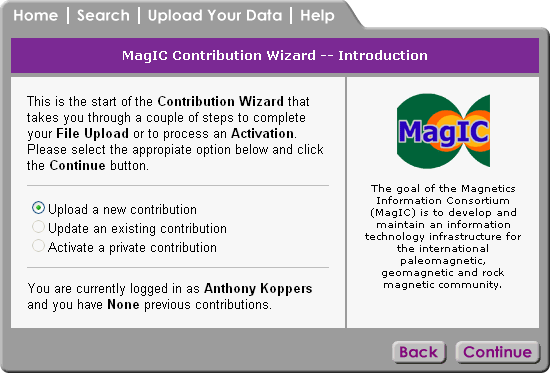
To proceed, you need to select the appropriate option:
Select the New contribution option if you are not going to update one of your existing contributions, or if this is your first contribution to the MagIC database.
Update an Existing Contribution
When you choose to update an existing contribution, you must upload the ASCII text file (*.txt) and Microsoft Excel file (*.xls) associated with the contribution. In most cases, an update will be necessary if some of the information in the existing contribution has been changed, or information has been added. You will be given a list of your previous contributions on the Reload Previous Contribution page. Select the contribution you wish to edit.
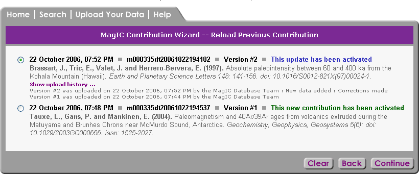
Changes will take effect immediately upon completion of the contribution process, and will be available for users to view. If your contribution is listed as In Progress on the Reload Previous Contribution page, it is not yet available for users to view, since the final confirmation page was not reached on your previous contribution visit. You must complete the entire process in order for your contribution to be available for users to see.
The Reload Previous Contribution form allows you to select one of your existing contributions to update.
A list of your existing contributions is given, with the most recently updated or created first. Contributions are grouped five per page, so if you have made more than five contributions, you will need to use the page navigation links at the bottom of the form to locate the desired contribution.
Each contribution is listed with the date contributed or updated, along with a unique identifier string and the contribution's status. A status of Completed indicates that you completed the entire process for that contribution, and it is currently available for users to view in search results. In Progress indicates that some steps in the process have not yet been completed for that contribution, so in order for users to view it, it must be completed. Updated indicates that the contribution was completed at some point, and that you have subsequently updated some of its data.
Other information is provided to help you differentiate your contributions. Each citation to which the contribution is linked is listed in the standard citation format, including its author(s), year published, title, and journal and DOI information, if applicable.
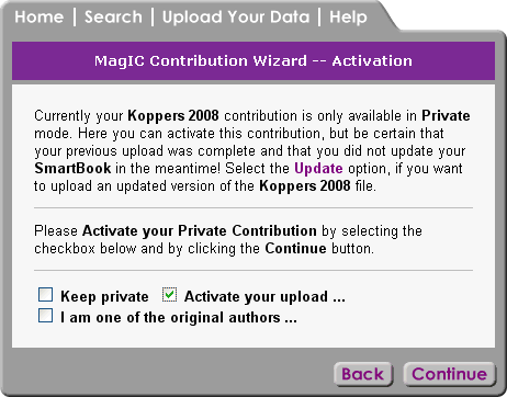
Activate a Private Contribution
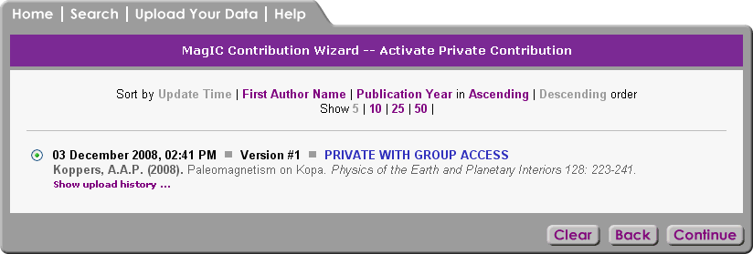
If this is your first contribution to MagIC, you will only be able to select the New contribution option.
All steps in the contribution process, along with the final confirmation step, must be completed in order for your contribution to be made available to users of the database. Once your contribution is in the database, you may update it at any time. If you do not complete your contribution, it will be removed from the database and you will need to upload it again.
In order to make a contribution, you must first log in. If you do not yet have a username and password, select the "login" option at the top right of your main browser window. From there, you may create a profile, username, and password.
Select the New contribution option if you are not going to update one of your existing contributions, or if this is your first contribution to the MagIC database.
When you choose to update an existing contribution, you must upload the ASCII text file (*.txt) and Microsoft Excel file (*.xls) associated with the contribution. In most cases, an update will be necessary if some of the information in the existing contribution has been changed, or information has been added. You will be given a list of your previous contributions on the Reload Previous Contribution page. Select the contribution you wish to edit.
Changes will take effect immediately upon completion of the contribution process, and will be available for users to view. If your contribution is listed as In Progress on the Reload Previous Contribution page, it is not yet available for users to view, since the final confirmation page was not reached on your previous contribution visit. You must complete the entire process in order for your contribution to be available for users to see.
2.1.2 Logging In
You must be logged in to make or update a contribution to MagIC. If you are not currently logged in, you will be automatically taken to the User Authentication screen, where you can enter your username and password. From there, you will be taken to the next step in the contribution process.
If you have not yet created a profile, you may follow the appropriate link from the User Authentication screen or click on the Register tab in the main browser window. This will take you to a simple form to enter your contact information and to create a username and password. The identification of contributors and their addresses is an integral part of scholarly data archiving and this information is continuously updated in the EarthRef.org address register. EarthRef.org does not distribute address information to third parties. You may read the entire EarthRef Privacy Policy by clicking on the Disclaimer link from the home page.
Some of the contact information given in your profile will be displayed when a user views your contributions, and from Mailing List searches.
2.1.3 Uploading Files
Two files must be uploaded for each contribution, and both are output from the MagIC Console Software. One file is a Microsoft Excel (*.xls) file, which contains a spreadsheet for each table in the database into which your data will be inserted. The other is an ASCII text (*.txt) file containing information that the upload programs need to be able to add your information to the database.
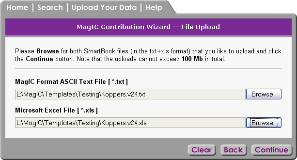
Uploading a file is accomplished in the standard fashion through your browser. Clicking the Browse... button will cause a dialog box to display, allowing you to browse for the desired file on your local computer or network. Once the file is selected, the file name will be automatically filled in beneath the upload field.
If either of the required files is missing from the upload, you will get an error message asking you to upload both files. In addition, if one of the files has become corrupted and can not be read, your upload will not be possible and you will receive an error message.
After clicking the Continue button, you will immediately see a progress bar showing the status of your upload. Because MagIC contribution files may contain several thousands of records and may therefore be very large, the file upload may take a moment. Please do not click the Continue button a second time since this will force the upload procedure to begin again and will delay your upload.

Upon successful upload, you will automatically be taken to the next step in the contribution process.
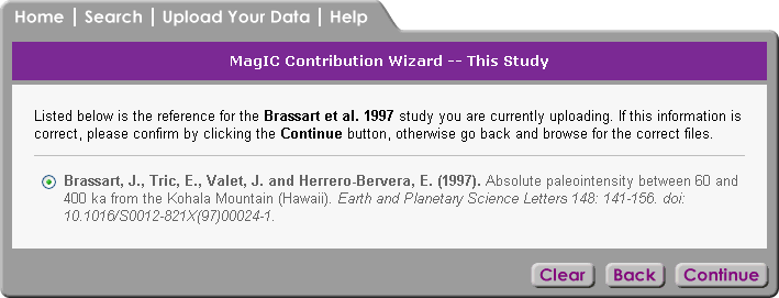
2.1.4 Selecting Main Reference ''This Study'' for Your Contribution
Upon successful file upload, you must first verify the main reference to which your contribution will be linked. If an exact match to the reference is found in the database (either by DOI or author list, year, and title), or the Contribution Wizard did not find any similar matches, you will see a screen like the one below in which one reference is listed. You need only click the Continue button to verify that this is the correct reference.
2.1.5 Selecting Additional References
After you have verified the main reference (This study) to which your contribution will be linked, the Contribution Wizard will process all other reference information included in your uploaded files. As with the main reference, the Wizard will attempt to find exact matches to the references.
If all references are found in the database (either by DOI or author list, year, and title) and no errors are found, you will not need to verify any information. Instead, you will automatically be taken to the next step. If neither an exact match nor similar matches are found in the database, the Contribution Wizard will insert the new reference.
If, however, the Contribution Wizard can not find an exact match but finds similar references, you will see it listed with one or more possible existing database matches, followed by the reference in your contribution. In most cases, there may only be a slight spelling or other variation between the existing reference and the one in your contribution, and you will need to verify that the highlighted reference is indeed the correct one to which your contribution should be linked. The Contribution Wizard tries to find the best match to your contribution's reference, but you must confirm the reference before proceeding.
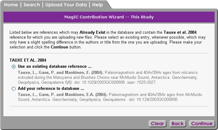
It is always best to select the existing database reference, even if you find slight variations in the spelling. This is because other data in the database may already be linked to it, and the existing reference data will most likely be much more complete than the reference in the contribution file. You may contact EarthRef.org to update the variation in the database. If you choose to add the new reference instead of using the existing one, the reference data that you provided in the MagIC software will be inserted into the database.
Occasionally, there is some data missing from the uploaded file because it has not been completed in the MagIC software prior to the creation of the upload files. In this case, you will see any problem references listed at the bottom of this screen to alert you to the fact that these references will not be matched to your contribution. It is best in this case to refer to your data in the MagIC program and to complete it as best you can. Once fixed, you may return to the Contribution Wizard to update the contribution. You may, however, choose to continue without correcting the references and update the contribution at a later time. Until then, your contribution will not be linked to the problem references.
2.1.6 Selecting Mailinglist Entries
Your data for people associated with the contribution you are uploading will be inserted into the EarthRef.org address book. The Contribution Wizard will perform a check to see whether these individuals already exist in the database. If a match is found for each individual, or no similar entries already exist, the mailinglist data will be automatically processed and you will not see this step.
If, however, an exact match can not be found for one or more individuals, and one or more similar entries are found, you will be asked to select the best match for each individual. As with the reference data, the difference between the information in your contribution and that in the database may be a simple spelling difference. If that is the case, it is always best to select the existing entry, as its data will be more complete, and it may already be linked to other data in the database. You must select the most appropriate entry and click the Continue button to process these records.
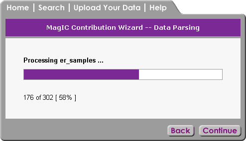
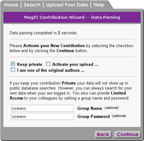
2.1.7 Data Parsing
Most of the data in your contribution (aside from reference data) will be processed in the Data step of the Contribution Wizard. In most cases, this will consist of inserting thousands of records into many database tables, which can take several minutes.
So that you will know where in the data processing stage the Contribution Wizard is, you will see a status bar like the one in the screen below. For each table in your contribution files, you will see a status bar indicating the current record being processed. The status bar image illustrates visually where each record lies, and below the bar is a numeric indication of the record.
If an error is found during the data processing, the processing will not continue. You will see a message indicating what the problem is so that you may fix it in your MagIC program data. Once fixed, you may return to the Contribution Wizard to update your contribution.
2.1.8 Activating Your Contribution
After processing is complete, you will see a confirmation message stating the number of seconds processing took, along with instructions for activating your contribution. Please note that even though your data has been inserted into the database, you must verify that you want to activate it by checking the checkbox on this screen. This is done to allow you to decide when your contribution will be activated. If, for example, an error was found at some point in the contribution process, or you decide you would like to update some of the data and re-upload the files, you may choose to wait until you have the updated data files to activate your contribution.
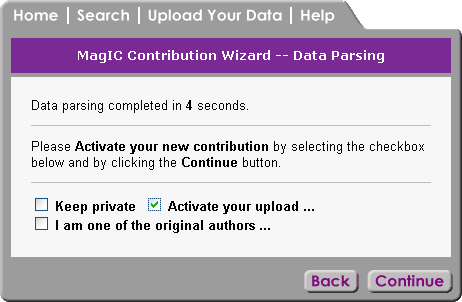
Activate Contribution with Global Access
If you continue without selecting the option to confirm the activation, your contribution will remain in the database temporarily, but will be unavailable for users to see. It will be removed from the database within 48 hours and it will not appear in your list of existing contributions.
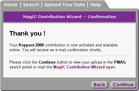
If you have checked the "Activate this contribution" checkbox on the previous screen, your contribution will be activated in this step, making your data available to users. You will again see a status bar indicating which table is currently being activated. The process will take only a few seconds.
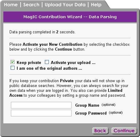
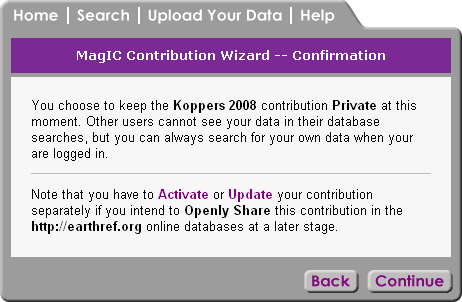
Keeping Contribution Private with Group Access
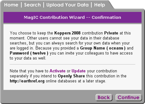
In this final step, a confirmation e-mail will also be sent to the e-mail address provided in your user profile, and will include a link to a summary page of your contribution data, a link to the main citation referred to in your contribution, and a reminder of your username and password.
Once activation has completed, you will see a confirmation message. At this time, your the contribution process is complete, and your data is available for users to see.
2.1.9 Summary Page
If you did not select the "Activate this contribution" checkbox on the previous page, your contribution will not be activated in this step, and instead of a status bar you will see a message alerting you to this fact. If you forgot to check the checkbox, simply click the Back button to return to the previous step, check the checkbox, and click the Continue button. The process will then proceed as described above.

2.2 Searching the Web Portals
Finding, collecting and downloading paleomagnetic and rock magnetic data from the MagIC Database is important for most users. In this Chapter we explain the different search functionalities you can find on the MagIC Home Page and in its Search Portals. For more detailed information on searching we refer to the Online MagIC Help Library at http://earthref.org/MAGIC/help.htm.
2.2.1 MagIC Website Home Page
Start by visiting the http://earthref.org/MAGIC home page, from where you can launch the PMAG and RMAG search portals, manage your own contributions, find important web links, a list of the most recent contributions, and read the latest news about paleo and rock magnetism.
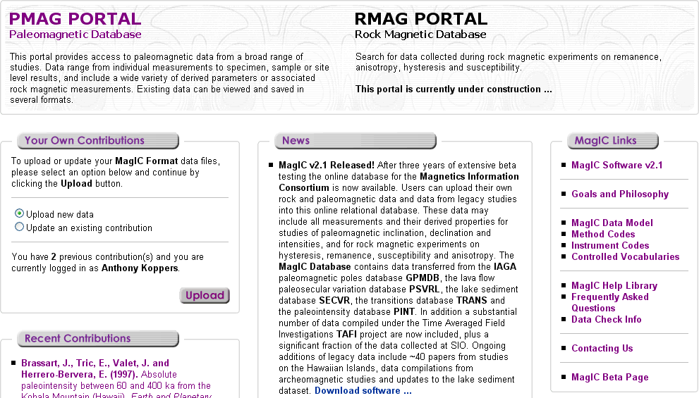
2.2.2 The PMAG Portal
The PMAG and RMAG web portals form separate entry points for paleo and rock magnetic searching. Although you can carry out different kind of searching, both portals interrogate the same underlying EarthRef.org and MagIC Databases. For this reason, you can find rock magnetic data when searching in the PMAG Portal and paleomagnetic data when searching in the RMAG Portal. The portals merely are different starting points that are tailored to the needs of either magnetic community.
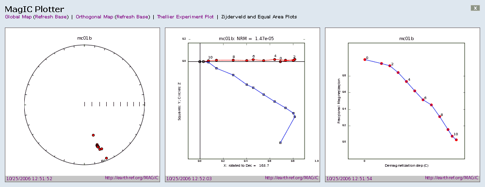
Below, we show you the resulting Measurement List from a particular drill down search in the PMAG Portal. As can been seen from this example, we drilled down from McMurdo to the actual measurements on Specimen mc01a. In this view of the data you can link back to the Tauxe et al. 2004 paper in the EarthRef.org Reference Database, you can use the links in the upper left of this listing to navigate back through your drill down history, and you can use the Save, Plot and Options pull down menus for more advanced functionality.
Note that the Units of the data are given between brackets in the Header of this table. All units are SI based, except for some fields, such as geological age. If you mouse over the headers, a longer explanation is given in a popup balloon. If you mouse over any of the cells in the table, a similar popup balloon is shown that contains the header information, as well as the basic information that is displayed in the left most column (experiment info in this example). This functionality will help you to better navigate larger data tables or when you show the table in Expanded View (see below).
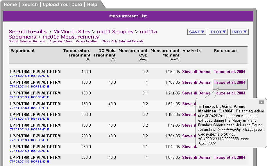
In the above example only data from the Basic View is shown. You can select the Expanded View from the links to the upper left. If you do so, all available data for each particular measurement are shown. In the near future you will have the ability to set your own Search Preferences, in which you can predefine what columns are shown in both the Basic and Expanded Views, and in what units you want to view your search results. For example, you will be able to set your preferences to always show ages in Ma and paleointensities in µT instead of the default T.
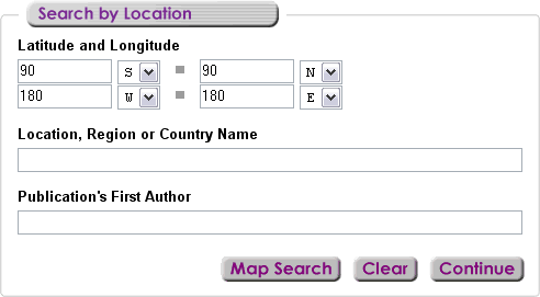
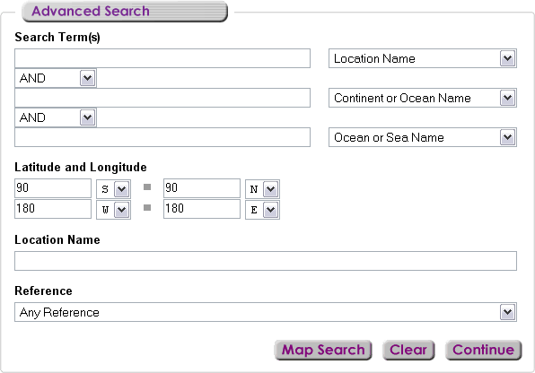
In the PMAG Portal one can search by location, which allows you to drill down from any location to the actual measurement data. You can do so by providing a lat-lon box, keywords to find a certain location by name, the last name of the first author, or a combination of these searches. You can also perform a map search by clicking on the Map Search button.
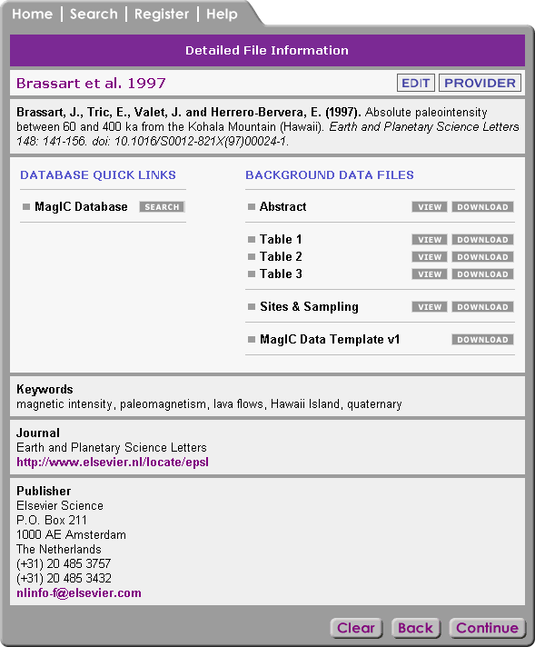
Searches by reference will provide you with a Detailed Reference Information table (see below) for a given publication. From this table you can view and download various Background Data Files, including the Microsoft Excel© and text versions of the MagIC SmartBooks. This table also provides Quick Links to the MagIC and other EarthRef.org databases, when these exist. In addition, a link may appear to the Provider of the publication, which redirects you to the Full Length HTML version of the paper on the publishers website. From here you can download a PDF of the publication, provided you or your institution has access to the journal or publication in question.
In the PMAG Portal you can also perform a more advanced search, which allows you to combine various Boolean searches terms. These terms normally are an accumulation of all other standard searches. You can also perform a map search by clicking on the Map Search button.
2.2.4 Plotting and Visualizations
Many Plotting and Visualization options are available through the Plot menu. In the plots and maps that you can generate at the MagIC Website all data from a single results table are included. If a results page contains more than one table, you can always Group Together the tables and make a new plot with all combined data. All plots can be saved as PNG (image) or SVG (scalable vector graphics).
These plotting tools will be expanded considerably in the future, allowing different kinds of experiments and data to be plotted, such as Rock Magnetic measurement plots (hysteresis loops, FORC diagrams, etc) and Stratigraphic Section and Drill Core plots. The ultimate goal is to make these plots and maps of good publication quality, to deliver them as SVG (already available), and to make the plotting more interactive so that you can access the results of different averaging scheme's or data selections.
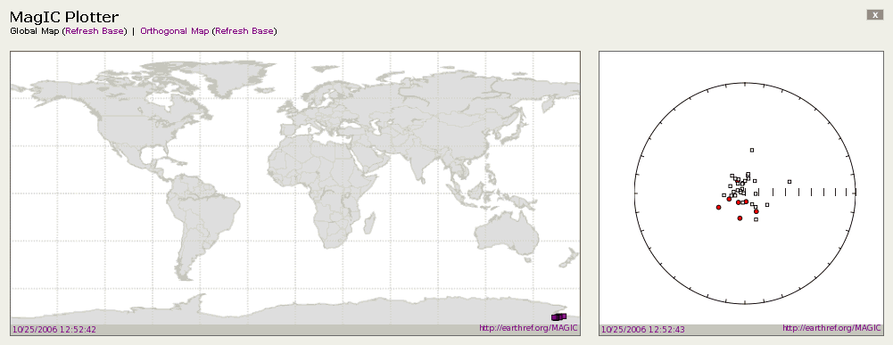
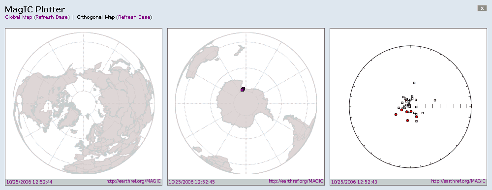
Global Maps and Orthographic Projections
On the Location, Site, Sample, Specimen and Measurement levels you can generate maps that plot their latitude-longitude positions. Global Maps (see the image above) are available as well as Orthographic Projections (below) in order to view data around the poles. Both map views are combined with an Equal Area plot.
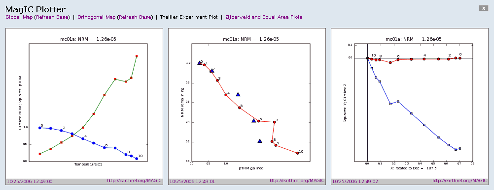
On the Measurement level you can plot various other diagrams, such as typical Zijderveld, Thellier and Arai plots. These plots (see below and next page for some examples) are drawn from the data residing in the database and provide a good view of the data itself and the quality of the experiments carried out.
2.3 Error Messages
2.3.1 Invalid File Type
The error "Invalid file type" will appear if one or both of the files uploaded are incorrect. The most common reason for this is inserting the Microsoft Excel file (*.xls) in the ASCII Text file (*.txt) upload field and vice versa. Simply click the Back button and insert the correct file into each field.
If you are certain that the correct file is in each upload field, a more serious issue may be the cause for this error. One of your files may be corrupt or can otherwise not be read correctly by the Contribution Wizard. In this case, it is suggested that you contact the webmaster for assistance.
2.3.2 Unable to Move File to Directory
The error "Unable to move [file] to [directory]" is a serious but uncommon error that may occur during contribution upload. It is a problem on the server side, and is not a consequence of a user action or corrupt file. When this error occurs, the webmaster is immediately notified, and the problem will be resolved. It is suggested that you contact the webmaster and you will be notified when the problem has been corrected.
2.3.3 Unable to Find File
The error "Unable to find [file]" occurs during data parsing when data is expected for a particular table but is not included in your contribution. The most common cause for this error is that it was not included in your input into the MagIC Console software. It is recommended that you return to the Console to complete your data input and then return to the Contribution Wizard.
If you are certain that the data input into the MagIC Console software is complete, please contact the webmaster with a description of the problem.
2.3.4 Missing Data for Reference
The error "Missing data for [reference]" occurs during the reference step when some data for a particular reference is incomplete. The missing data will be described with the error message. The most common cause for this error is that it was not included in your input into the MagIC Console software. It is recommended that you return to the Console to complete your data input and then return to the Contribution Wizard.
If you are certain that the data input into the MagIC Console software is complete, please contact the webmaster with a description of the problem.
3 MagIC Console Software
Getting your data organized, complete and ready to submit for a paper publication or ingesting into a database is a time-consuming job. We have developed the MagIC Console Software to aid you in your collation of paleomagnetic and rock magnetic data and to make the data ready for uploading in the MagIC database.
3.1 Introduction to the Standardized MagIC Data Format
Establishing an integrated paleomagnetic and rock magnetic database is difficult as we need to move large quantities of data into the MagIC database from both legacy and new studies. To address this challenge we have chosen an approach that makes the archiving of these data Synchronous with the Scientific Publication process and is entirely based on User Contributions. Around the time of publication each scientist has all relevant data for a publication at his fingertips and knows best how to deal with it. In fact, he probably went through a sustained effort to collect all measurement data (and most of the relevant metadata) to perform his or her scientific research. The MagIC Console Software is developed to aid the scientist to collate all information at this opportune time and to do so by making use of a Standardized MagIC Data Format.
3.1.1 What is a SmartBook?
We wish to tap into this process by supplying scientists with a tool that they can use to collect all data that are relevant to one particular publication (henceforth referred to as a project). Key to this approach is a standard Data and Metadata Template in the form of an Microsoft Excel© SmartBook in which they can enter their data and in which they can further process their data to eventually upload into the online MagIC database.
Because we use this standardized SmartBook protocols can be established around which scientists can build (or adapt) their (current) laboratory protocols. For example, they can streamline the collection of measurement data by enabling the export of standard MagIC Format Text Files that can be readily imported into the MagIC SmartBooks. Similar export functions can be established for various data reduction software and geomagnetic modeling codes. This approach significantly increases the flow of magnetic data into the MagIC database and circumvents labor-intensive data entry for individual scientists.
The MagIC SmartBook has been defined in a way so that it can store all measurements and their derived properties for studies of paleomagnetic directions and intensities, and rock magnetic experiments, such as hysteresis, remanence, susceptibility and anisotropy. The basic design of this SmartBook focuses on the work-flow in typical paleomagnetic and rock magnetic studies. This ensures that individual data points can be traced between actual measurements and their related specimens, samples, sites, locations, and so forth.
To make working with the MagIC SmartBooks more straightforward, we have developed the MagIC Console Software that, in addition to many other functions, contains an Import function for standard text files. This software helps you to Enter Data, it helps you to check the Correctness and Coherence of the data entries, and it helps you Prepare for Uploading your SmartBook in the MagIC database. Since the MagIC SmartBooks have been developed as Microsoft Excel© Files, most users will feel comfortable with the setup, which makes use of standard toolbars and dialogboxes.
3.1.2 Structure of the MagIC SmartBooks
The MagIC SmartBooks are standard Microsoft Excel© Workbooks that contain predefined tables stored in separate worksheets. There is an obvious hierarchy in these tables, where the EarthRef (ER) tables are the most general and are applied to other databases hosted under this umbrella website as well.
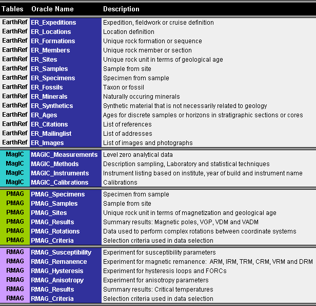
The four MagIC tables (measurements, methods, instruments and calibrations) are less general, but contain data and metadata that are common for typical paleomagnetic and rock magnetic projects. The PMAG and RMAG tables contain the most specialized, highly derived data.
3.1.3 MagIC Table Layout
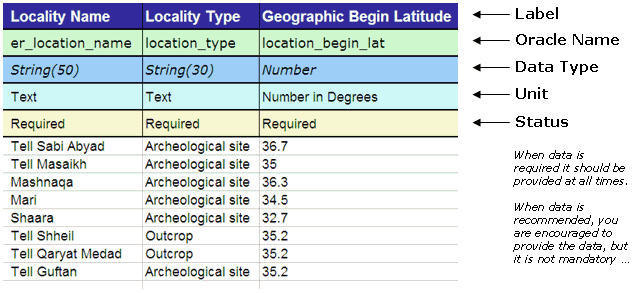
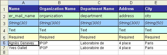
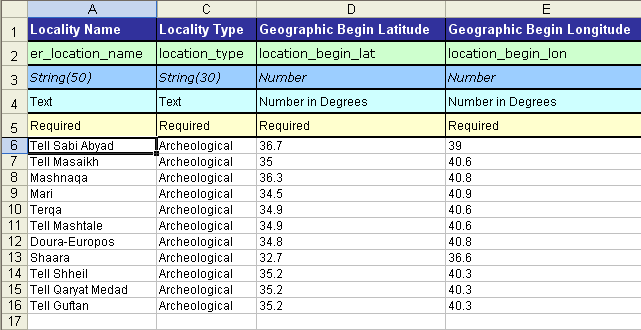
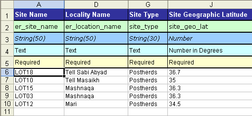
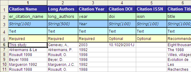
Each table is divided into several pre-titled columns. The first Five rows of each column characterize the data to be entered below the headings. The first row gives the Label of the column and describes the data to be entered (explanation in plain English). The second row displays the Oracle Variable Name associated to these data in the relational database and used by the MagIC Console Software. The third row indicates the Data Type and maximum length of text strings. The fourth row shows the expected Unit of the data. The fifth row indicate the Status of the data to show whether the data is required, recommended or optional. All five heading rows are fixed in the MagIC Data and Metadata definition, which is strictly maintained and versioned.
Upon opening a SmartBook in the MagIC Console Software they will be used to check the validity of the tables and columns residing in the Microsoft Excel© File.
3.1.4 Standard MagIC Text File Format
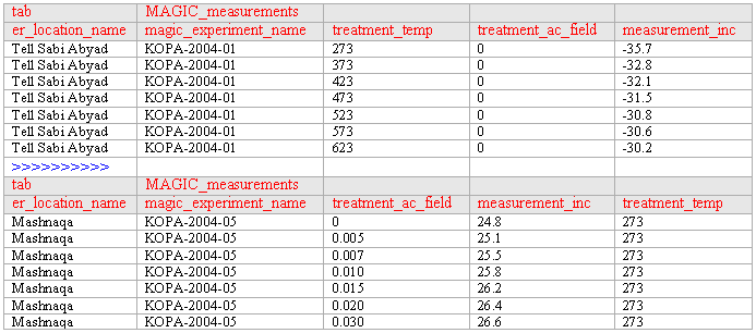
The MagIC Console Software has the ability to export and import Flat Text Files. To be able to easily transfer data between outside software packages, data collection computers and the MagIC SmartBooks, we have developed the Standard MagIC Text File Format. Experience shows that this is the most efficient way when dealing with large data sets. It allows you to quickly import these data into the MagIC SmartBooks without making mistakes. In the example below, we show how this text file is based on the layout of the table displayed above.
The Standard MagIC Text File Format starts out with two header lines (red fonts) indicating the delimiter used, table name and column names. Below these header lines, the data appears in the same order as indicated by the column names (black fonts).
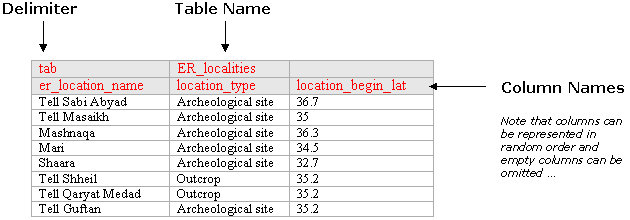
Possible delimiters include tab and pipe symbols. Note that single or double quotes around text strings are not required. You can also store multiple data blocks (for one project) in one text file, where each data block is stored according to the above rules but is separated by the standard >>>>>>>>>> divider. Since each block has its own header lines, in principle, you can store the results from different experiments or tables in one and the same Standard MagIC Text File. This will result in a text file that may look as follows.
3.1.5 Software Installation
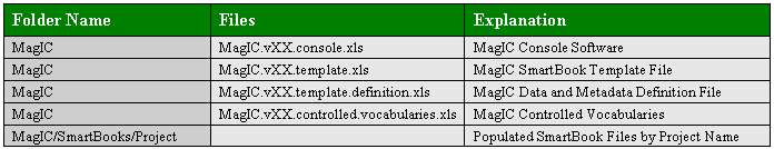
The MagIC Console Software does not work with a fixed directory structure. However, we recommend that you generate a main MagIC directory on your hard disk and that you store the populated SmartBook for each of your MagIC Projects in sub directories.
In the table below we have listed Four files that are required for a proper functioning of the MagIC Console Software. Note that each file has been named according to its current version, that is v20 or v24 (instead of vXX) for example.
3.2 Entering New Data
While populating the MagIC SmartBooks there are several possible approaches to put your paleomagnetic and rock magnetic data into these Microsoft Excel© Files. Here we will provide a guided explanation on how to populate the MagIC SmartBooks most effectively, using a top-down approach, where first the high-level data and metadata are entered, followed by more detailed magnetic measurement and derived data later on.
Note that this an example only that allows you to get familiar with the capabilities of and functions available in the MagIC Console Software. There may be better ways to go about this for certain special cases or data sets, as described elsewhere in this help library.
3.2.1 Overview of the Data Population Process
We start out by giving an overview of the MagIC Data Population process, which can be divided into four different parts. We will follow this general overview by a Step-by-Step Guided Explanation of the process.
Starting a New MagIC SmartBook
Entering the High Level Metadata
Entering and Importing PMAG and RMAG Data
The above 15 steps will be discussed in detail in the Step-by-Step Guided Explanation in the next help topic. Remember, however, that this is a generalized approach. Some steps may not be required (and thus can be skipped) because they are not relevant to your project. Therefore, it is especially important to always run the MagIC Wizard at the beginning of your data population session.
3.2.2 Step-by-Step Guided Explanation
1. Start the MagIC Console Software
2. Generate a New SmartBook File
4. Add Your Current Project Citation in the ER_citations Table (This Study)

5. Compile Methods Definitions for this Project
6. Compile Instrument Definitions for this Project
7. Add other Citations to ER_citations table
8. Add all Mail Addresses to ER_mailinglist Table
9. Define the Data and Metadata in the General EarthRef [ER] Tables
10. Add Age Data to the ER_ages Table
11. Add Measurement Data in the MAGIC_measurements table
12. Add Paleomagnetic and Rock Magnetic Data
15. Upload your SmartBook into the MagIC Online Database
3.3 Special Cases
There may be a few cases that require a special approach while populating the MagIC SmartBooks. In this Chapter we treat these special cases by briefly describing the issue and a possible solution.
3.3.1 When Requiring New Instrument Codes
If you cannot find the appropriate Instrument Code in the software, you can always create a new code by activating the MAGIC_instruments table and by clicking the Edit Data button on the MagIC Toolbar. Continue by clicking the New Record button and fill out all fields. After uploading your files this new code will be reviewed and, if this new code is acceptable, it will be added to the Controlled Vocabulary listing of instruments.
3.3.2 When Entering More Than 65,000 Measurement Data Records
The user cannot add more than 65,000 data records in a single table due to the limitations of the Microsoft Excel© worksheets. However, there is one exception made for the records of the MAGIC_measurements table. In this table you can import as many measurements as required. If the software detects more than 65,000 records, it will automatically generate a table named MAGIC_measurements2, and so on.
3.3.3 When Starting Data Population from Measurement Files
It may be quite common that you start data population with a measurement file, which has been stored in the Standard MagIC Text File Format. When pursuing this route, first import all these text files into a SmartBook that have been prepared by applying the first six steps described of a typical file upload procedure. Follow this by running the Synchronize Names function from the Special menu to pre-fill the names of all Locations, Sites, Samples and Specimens (and others) throughout the tables of the SmartBook. Now you only have to complete these tables with some extra data and metadata.
When new records are added to these tables using the Synchronize Names function, they will appear in highlighted "light blue" and "pink" cells for easy detection. The originating data records are highlighted "purple" as well. You can remove the formatting again by pressing Ctrl Shift S or it will automatically be removed when you run the Prepare for Uploading function.
3.4 Examples
In this Chapter we will present examples of a few common tasks you most likely will perform during the uploading of your data. The examples are meant to give you a step-by-step visual summary of what you will have to do to complete these tasks.
3.4.1 Entering References in the ER_citations Table
In every SmartBook you have to enter the bibliographic information for your current contribution to the MagIC Database. You may also need to add references for publications from which you have been compiling additional data. Typically you would follow the next sequence of actions ...
3.5 Function by Function
3.5.1 Operations Menu
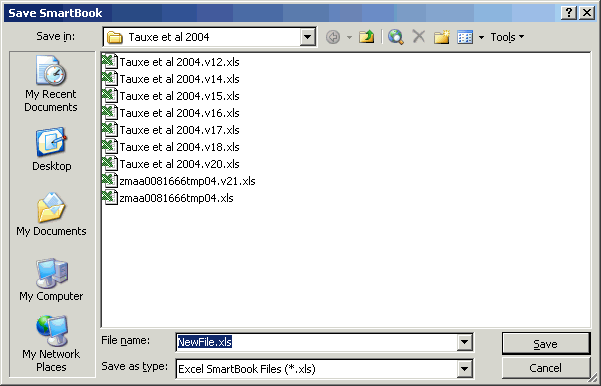
To open a new MagIC SmartBook file, choose the New File ... command (or ctrl-N) in the Operations menu. In a dialogbox you will be asked to Save the SmartBook File under your name of choice. The NewFile.xls is a default name that you can overwrite, as necessary. When clicking on the Save button, a new and empty MagIC SmartBook is created with 30 predefined tables (worksheets).
To open a MagIC SmartBook, choose the Open Existing File ... command (or ctrl-O) in the Operations menu. In a dialogbox you will be asked to browse and select the SmartBook file you would like to re-open in the console software.
Select the Close ... or the Close All ... commands in the Operations menu to close the active MagIC SmartBook file(s). Upon closing the console software will ask you to save the file(s) first.
Click the Save ... command (or ctrl-S) in the Operations menu to save the active MagIC SmartBook file. This command has the same functionality as the Save button on the left-hand side of the toolbar itself. Clicking Ctrl Shift and the Save button [Windows platform only] will save the SmartBook file after cleaning up and reformatting all tables.
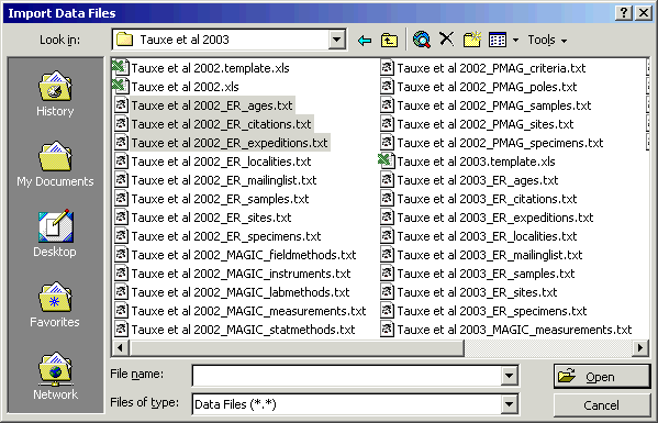
Click the Import Data Files ... command (or ctrl-M) in the Operations menu to import Standard MagIC Text Files with data to include in the SmartBook tables. An Import Data Files dialogbox appears in which you can browse for these standard text files. You can select multiple text files by holding down the Ctrl or Shift keys [Windows platform only]. When clicking on the Open button, the selected file(s) will be opened and the data will be imported into the MagIC SmartBook tables.
If the data in the Standard MagIC Text File to import don't have the expected format, an error message will appear. Note that data in a column with a misspelled Oracle Name will be ignored while importing the data. The software will give you an error message.
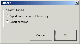
Click the Export command (or ctrl-E) in the Operations menu to export Standard MagIC Text Files. You will be asked to export data for the current (active) table only, or to export all tables in the entire MagIC SmartBook file. All data will be exported into a single tab delimited text file with your chosen file name.
To automatically Import data and immediately Prepare for Uploading (see above) choose the Batch Processing ... command from the Operations menu. You will be asked to select one or more Standard MagIC Text File(s) [multiple files are only allowed on the Windows platform] after which the data processing starts without any user interaction. If errors occur during the five Data Checks they will not cause a prompt, but instead they will be written to an Error Log. This is an efficient option if you prepare Standard MagIC Text Files outside of the MagIC Console Software and you only want to pass your data through the console to make them ready for uploading. Since all checks get performed without any interrupting for your entire data contribution, the error logs give you a good overview where you should improve on your data and metadata collection.
When all data have been entered in the MagIC SmartBook choose the Prepare for Uploading command (or ctrl-F) in the Operations menu. You will be asked for be asked for a confirmation. If you click the Yes button, five Data Checks will first be performed before the data is saved in a single tab delimited text file. This may take several minutes, depending on the complexity and the amount of data stored in the SmartBook. Clicking the No button will cancel this action.
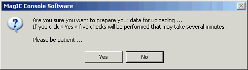
The five Data Checks include a SmartBook integrity check, a check for orphaned data, a general data check, a specific data check (for longitudes, citation style, data ranges, etc.) and an integrity check for all related data fields. If one of these checks returns an error, the Prepare for Uploading command will ask you to edit (or add) certain data and metadata. If you do not edit the particular field at this stage, you will cancel the Prepare for Uploading action.
After the succesfull completion of the Prepare for Uploading command you are ready to upload your data on the MagIC Website. Goto http://earthref.org/MAGIC/upload.htm or click on the Upload Into MagIC Database command in the Operations menu.
3.5.2 Special Menu
The widths of all columns in a table may be automatically adjusted to Autofit the five header rows using the Autofit Columns command in the Special menu.
To clear all the data in a table (worksheet) choose the Clear Table command in the Special menu. You will be asked for a confirmation.
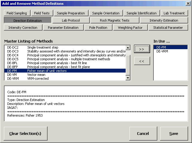
Add and Remove Method Definitions ...
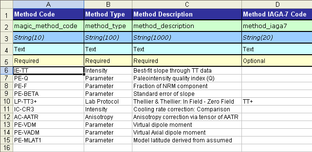
Each MagIC Project only requires a limited number of Method Definitions. By clicking on the Add and Remove Method Definitions ... command in the Special menu you can generate a list of Method Codes that describe the methods used in your project, including field sampling techniques, lab protocols, parameter estimations, and more (see the buttons at the top of this dialogbox for a complete list of categories). The Method Codes that are currently stored in your MagIC SmartBook file are listed in the In Use ... list box shown on the right-hand side.
You can Add new Method Codes by first selecting a method from the master listing of methods list box on the left-hand side, followed by clicking the right-pointing Double Arrow button. Show different categories of the Method Codes in this master listing by clicking on the Category Buttons in the top of this dialogbox.
You can Remove the Method Codes one-by-one by selecting the code in the In Use ... list box, followed by clicking the other left-pointing Double Arrow button. You can remove all methods at once by clicking on the Clear Selection(s) button. The program will ask you for a confirmation.
When you are finished compiling your list of Method Codes, click the Save button. This action will store all newly assigned Method Codes in the MAGIC_methods table, and it will add the appropriate references to the ER_citations table.
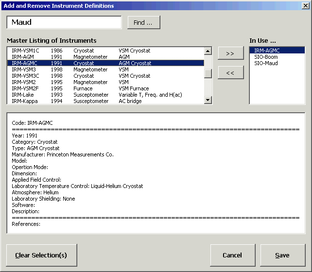
Add and Remove Instrument Definitions ...
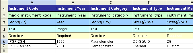
Each MagIC Project only requires a limited number of Instrument Definitions. By clicking on the Add and Remove Instrument Definitions ... command in the Special menu you can generate a list of Instrument Codes that describes the instruments used in your project. The Instrument Codes that are currently stored in your MagIC SmartBook file are listed in the In Use ... list box shown on the right-hand side. The Instrument Codes should all start with an abbreviation indicating the host institution.
You can Add new Instruments by first selecting an instrument from the master listing of instruments list box on the left-hand side, followed by clicking the right-pointing Double Arrow button. You can search for Instruments by typing in (part of) a name in the top textbox, followed by clicking on the Find ... button.
You can Remove the Instruments one-by-one by selecting the code in the In Use ... list box, followed by clicking the left-pointing Double Arrow button. You can remove all instruments at once by clicking on the Clear Selection(s) button. The program will ask you for a confirmation.
When you are finished compiling your list of Instruments, click the Save button. This action will store all newly assigned Instrument Codes in the MAGIC_instruments table, and it will add the appropriate references to the ER_citations table.
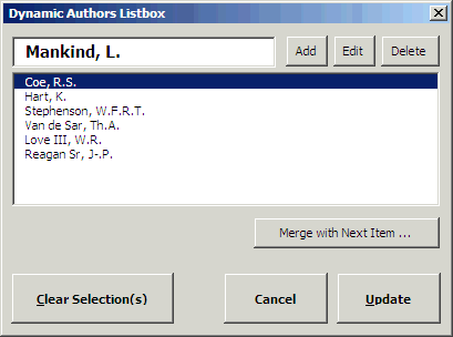
Some names, such as Location, Site, Sample and Specimen names appear in more than one place in the MagIC SmartBooks. Use the Synchronize Names function in the Special menu to automatically pre-fill these names throughout all the tables. This requires that you have at least filled out these names in one of the SmartBook tables. When new records are added to these tables they will appear in highlighted "light blue", "pink" and "purple" cells for easy detection. You can remove the formatting again by pressing Ctrl Shift S or when you Prepare for Uploading.
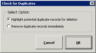
You can detect and remove Duplicate Data Records in your tables by choosing Remove Duplicate Data Records from the Special menu. It is recommended that you first Highlight duplicate records. If you select this option, the potential duplicates get highlighted with an "orange" color. If you opt to Remove the duplicates immediately, the duplicate record(s) will be deleted from you table instead, while the first instance will be retained. Note that this action cannot be undone.
You can detect and remove Empty Data Records by choosing Remove Empty Data Records from the Special menu. You will be asked to remove empty data record for the current (active) table only, or to do so for all tables in the entire MagIC SmartBook file. Note that this action cannot be undone.
![]()
Combine Two Similar Data Records
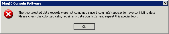
In some cases, tables may have sets of data records that are very similar, where they for example have the same sample number, but one data record (i.e. row) contains inclination and declination data, and another one only paleointensity data. These data records could be combined (i.e. merged) into one record. In order to do so, select two similar data records in a table and choose Combine Two Similar Data Records from the Special menu. If there are no data conflicts, the rows will be combined on the first row and the second row gets deleted. If the data cannot be combined, an error message is displayed and the data conflicts are highlighted in "orange" colors. To select two rows in your table, push the control key and click on any cell to select the first and second row. Note that this action cannot be undone.
To verify that the data in one table have the expected format, choose the Check Data Records command in the Special menu. You will be asked to check data for the current (active) table only, or to check all tables in the entire MagIC SmartBook file.
You can also verify whether specific data (like latitudes, longitudes, citations, magnetic moments, paleointensities, flags) have the expected format and range of values. Some automatic repairs will be performed in the background (e.g. recasting longitudes from the -180/180 to the 0/360 notation) during this data check, other checks may return error messages. To perform this function, choose the Check Specific Data Records command in the Special menu. You will be asked to check data for the current (active) table only, or to check all tables in the entire MagIC SmartBook file.
To validate whether data in one table are correctly related with other data tables in the SmartBook file, choose the Check Data Integrity command in the Special menu. You will be asked to check data for the current (active) table only, or to check all tables in the entire file. This action will search each table for existing relations and it will check them against their parent tables. If a relation is broken (i.e. the parent record does not exist, or you misspelled the daughter or parent record) then an error will occur. You will be asked to edit certain data and metadata.
3.5.3 Data Entry and Editing Dialogbox
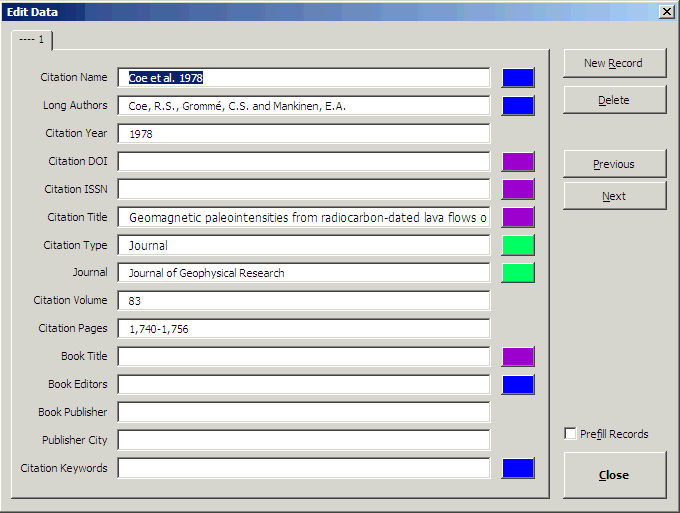
There are various ways to enter your data in the MagIC SmartBooks. One of these methods is the Edit Data option (or Ctrl Shift D) that you can find on the main MagIC Toolbar. In this dialogbox you can enter, edit and delete data on a record-by-record basis. If you want to edit an existing data record, first select the data record you want to edit by selecting any cell in its row in the Microsoft Excel© table, followed by clicking on the Edit Data button. You can also Double-Click on the cell. The complete record will be loaded in the dialogbox and will be ready for editing. Use the numbered Tabs on the upper left-hand side to show additional fields, if more than 15 data fields are available for a record.
Note that you can edit all fields, but your changes will only be applied to the MagIC SmartBook when you click the Close button, when you move through your records by using the Next and Previous buttons, or when clicking the New Record button. Temporary changes can be undone by Canceling the dialogbox.

To add a new record click the New Record button. With this action a new record is inserted at the bottom of the active table.
To delete the currently loaded data record from the MagIC SmartBook table click on the Delete button. You will be asked for a confirmation. Deletions cannot be undone.
To move between adjacent data records click on the Previous or Next buttons. You can also make use of the Alt P and Alt N shortcut keys for faster navigation. Note that each data record preloaded in the Edit Data dialogbox is checked automatically, when you move to the next or previous data record, or when closing the dialogbox.
If you checked the Prefill Records checkbox, this new record will be pre-filled with the data from the currently-selected data record in the active table. Use this functionality when adding data records that have the majority of their data field entries in common. This might significantly improve the speed of data entry for larger data sets.
Tab Navigation and Hot Buttons
To facilitate the efficient editing of your data in the Edit Data dialogbox, you can make use of the colored Hot Buttons on the right-hand side of this dialogbox, which will open Pop-Up dialogboxes (see below for two examples). These Hot Buttons can be divided into 3 different categories:
The Purple Buttons will provide you with a larger edit box to enter Long Text Entries.
Lists and Controlled Vocabularies
The Light Green and Light Blue Buttons provide you with Shortlists to select a single predefined item or multiple items (see example below). In case of the Light Blue Buttons your selection will create links towards other data tables in the MagIC SmartBook file. To select multiple items simply click on as many records in these lists as required.

Dark Blue Buttons help you enter names of Authors and Editors in the ER_citations table in the proper format, as expected for the MagIC and EarthRef.org databases. Use the add, edit and delete buttons to enter the correct author and editor information. These Dark Blue Buttons also give interactive dialogboxes to allow you to enter multiple keywords, ocean names, country names, etc.

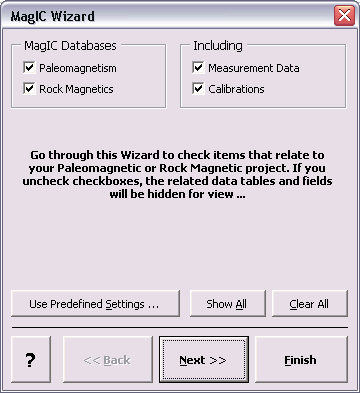
3.5.4 MagIC Wizard
Depending on the type and characteristics of a study, certain fields in the MagIC SmartBook tables may not be relevant and should be hidden. The MagIC Wizard can be launched from the MagIC Toolbar (or Ctrl Shift W) and allows you to customize the SmartBook in three steps. In effect, this tool will temporarily hide some tables and columns from view in Microsoft Excel© depending on the options you selected. Note that the selections made in the Wizard are only applied after clicking the Finish button.
In each of the three wizard steps (see next page an example) you can Check or Uncheck the checkboxes that are relevant to your study. As you will see, these options go from general in the first step to detailed in the following steps. While unchecking these checkboxes, the wizard may uncheck other checkboxes by default. You can always recheck these checkboxes again, if you require that data to appear in your MagIC SmartBook file.
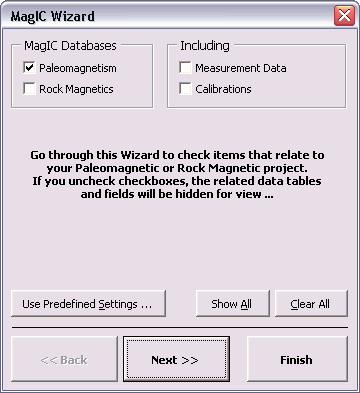
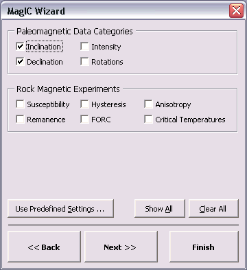
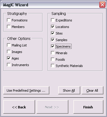
Show All and Clear All Buttons
You can show all fields again by clicking the Show All button in the Wizard, followed by clicking the Finish button. Alternatively, you can click the Clear All button to uncheck all checkboxes.
You can also use Predefined Settings to more easily apply the needed settings. When you click the Use Predefined Settings ... button, another dialogbox appears with options like Classical Directional Study, Classical Intensity Study, Modern Paleomagnetic Study, Modern Stratigraphic or Drill Core Study, and so on.
3.5.5 Navigating a SmartBook
The data in each table may be sorted in an ascending order using up to three columns as keys. To sort on only one column, select any cell in this column and click on the Sort button. To select two or three columns for sorting, push the control key and click on any cell to select the first, second and third column, and then click on the Sort button. The order in which you selected the sorting columns also determines the order in the sorting keys. Note that this action cannot be undone.
With this button you can move to the First Column in the active table without scrolling vertically. You can also use Ctrl Shift Home on your keyboard.
To move multiple columns use the left and right buttons on the toolbar, or hold down the Ctrl Shift keys while using the Arrow Keys on your keyboard. This will allow you to move from one set of columns that are visible in the active Microsoft Excel© window to the next (or previous) set, showing you at least one or two columns overlap. These actions do not cause any vertical scrolling.
With this button you can move to the Last Column in the active table without scrolling vertically. You can also use Ctrl Shift End on your keyboard.
Use this menu to navigate between different Tables in the active MagIC SmartBook file. This pull down menu will be automatically updated every time you switch between different SmartBooks using the SmartBooks toolbar menu (see below).
You can switch between different MagIC SmartBook files using the SmartBooks toolbar menu. If you activate another file through this menu the Tables menu (see above) will be automatically updated.
3.5.6 Text Tools
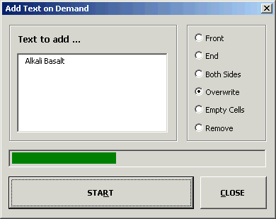
Select the cells to which you want to add some text or which ones you which to remove or overwrite with some other text, in batch mode. Select the Add Text Tool option from the Text Tools menu. In this tool first type the Text to add ... and then select the Action you want to perform on the right hand side. Apply these settings by clicking on the Start button. Note that this function cannot be undone.
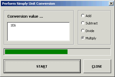
Select the cells on which you want to perform some simple conversions. Then select the Number Conversion Tool option from the Text Tools menu. Type in the Conversion value ... and select one of the actions on the right hand side. Click on the Start button to start applying the conversions. You only can perform one operation at a time.
Select the cells from which you want to remove all spaces. Select the Remove All Spaces option from the Text Tools menu. Note that this function cannot be undone.
Select the cells from which you want to remove extra spaces only. Select the Remove Extra Spaces Only option from the Text Tools menu. This function will remove all Double Spaces and any existent Leading and Trailing Spaces. Note that this function cannot be undone.
Select the cells from which you want to remove all characters with the exception of numbers. Select the Remove All Characters option from the Text Tools menu. This function will remove all Non-Numeric Characters, except for the "-" (minus) and "." (period) symbols, so that it leaves only numeric values. It will also remove all Spaces. Note that this function cannot be undone.
Remove Parentheses and Brackets
Select the cells from which you want to remove all parentheses and brackets. Select the Remove Parentheses and Brackets option from the Text Tools menu. This function will remove all the "( )", "[ ]" and "{ }" symbols. Note that this function cannot be undone.
Select the cells from which you want to remove strange symbols. Select the Remove Strange Symbols option from the Text Tools menu. This function will remove the "~!@#$%^&*_`'|<>? =" symbols and the "tab" character. Note that this function cannot be undone.
Select the cells from which you want to remove line feeds and carriage returns. Select the Remove Line Feeds option from the Text Tools menu. Note that this function cannot be undone.
Select the cells for which you want the text to appear in all lower case. Select the Make All Lower Case option from the Text Tools menu. Note that this function cannot be undone.
Select the cells for which you want the text to appear in all upper case. Select the Make All Upper Case option from the Text Tools menu. Note that this function cannot be undone.
Select the cells for which you want the text to appear in normal case, meaning that only the first letter of the text will appear in upper case, while the remainder will appear in lower case. Select the Make Normal Case option from the Text Tools menu. Note that this function cannot be undone.
Select the cells for which you want the text to appear with each word having normal case. This means that the first letter of each word in the text will appear in upper case, while the remainder of these words will appear in lower case. Select the Make Every Word Normal Case option from the Text Tools menu. Note that this function cannot be undone.
3.5.7 MagIC Help Menu
Select the Metadata and Data Model option from the MagIC Help menu to launch your browser and to review the current metadata and data definition. When entering this web page you will first see an overview of all Tables that define the MagIC SmartBook files. Click on a Table Name to view the definitions of the Records (columns) that define these tables, including short explanations and examples. Note that this function is equivalent to following the http://earthref.org/MAGIC/metadata.htm link. On this web form you can also do a free text search.
Select the Method Codes option from the MagIC Help menu to launch your browser and find a listing of Method Codes that currently are in use. On this page you will find a list of method types (or groups) for which we have defined codes. Please click on one of these method types to retrieve a list of relevant Method Codes and their definitions. Note that this is a dynamic list. With every new version, new Method Codes may have been added to the system, and will show up in these listings. This function is equivalent to following the http://earthref.org/MAGIC/methods.htm link. On this web form you can also do a free text search.
Select the Instrument Codes option from the MagIC Help menu and find a listing of Instrument Codes that currently are in use in the MagIC Database. Please click one of these codes to view their definitions. Note that this is a dynamic list. Every time a user adds new data, new Instrument Codes may have been added to the system, and will show up in these listings. This function is equivalent to following the http://earthref.org/MAGIC/instruments.htm link. On this web form you can also do a free text search.
Select the Controlled Vocabularies option from the MagIC Help menu to find a listing of all Keywords that can be used when entering your data using the MagIC Console Software. On this page you will find a listing of Controlled Vocabularies for which we have defined keywords. Please click on one of the listed vocabularies to retrieve a list of (optional) keywords. This function is equivalent to following the http://earthref.org/MAGIC/shortlists.htm link. On this web form you can also do a free text search.
3.7 Known Bugs and Workarounds
This section contains a list of know Bugs and Workarounds to solve these problems. If you encounter new bugs, we would appreciate it if you could email us and provide us with information that describes the circumstances under which you encountered the problems. Thanks!
3.7.1 Object Library Not Registered (Macintosh OS X)
If you encounter an Object library not registered error message on Macintosh© OS X systems, your Microsoft Office© installation contains a corrupt library/preferences/Microsoft/Office Registration Cache X file. Open this file in a text editor, where you should remove all text and save it. Finish by locking this file and restarting the Microsoft Excel© application. The locking of this text file is most essential, otherwise the problem will re-occur.
3.7.2 Appearance of Blank MagIC Toolbar (Macintosh OS X)
When starting the MagIC Console Software by double clicking on the MagIC.vXX.console.xls file in the Finder or from the Desktop, the software might start up displaying a blank MagIC toolbar. This problem can be circumvented by first launching the Microsoft Excel© application itself, followed by opening the MagIC.vXX.console.xls file through the File # Open menu. In some cases, updating to Service Pack 1 will remedy this problem as well.
4 Importing Data With PmagPy and MagIC.py
The MagIC Console software allows entry of data directly into an Excel Smartbook. However, the work flow for a typical paleomagnetic study involves taking samples in the field, analyzing specimens in the laboratory and interpreting those measurements in a variety of ways. Individual laboratories use a variety of custom software packages to create plots and tables that are suitable for publication from the measurement and field data. Measurements are made on specimens which are part of samples which are part of sites and this context must be preserved explictly in the MagIC database tables. Also, measurements can be done on a variety of instruments, under different conditions of pre-treatment, measuring temperatures, frequencies, orientations, etc. These details must also be preserved in the database for the measurement data to have any value. To facilitate the process of analyzing and importing paleo- and rock magnetic data and meta-data into the MagIC console, we have written the PmagPy software package.
PmagPy is written in the Python Programming Language. Python is flexible, freely available, cross platform, widely used and well documented and much easier to read and learn than Perl. It has many numerical or statistical tools 3D visualization is improving all the time. And it is free. As of this writing, PmagPy comprises 135 programs which perform a variety of tasks from simple calculations to creating complicated plots. These call on functions in several modules: the plotting module, pmagplotlib does the heavy lifting for creating plots and pmag has most of the functions performing calculations. Details on how to use the complete software package and the source code are available through the PmagPy home page.
PmagPy programs are called from the command line and uses switches to set key parameters. Most paleomagnetists are not Unix oriented and dislike the command line interface. For this reason, we have written a graphical user interface (GUI) called MagIC.py. MagIC.py allows importing of field and measurement data for a variety of laboratory conventions into the MagIC format. It also allows plotting and interpretation of the data and preparation of all the data files into to text file that can be directly imported into the MagIC console.
4.1 Installation of PmagPy
Python can be painful to install (but so can all other programming environments). The Enthought Python Distribution is a comprehensive version that contains all of the packages used by PmagPy. It is also relatively straight-forward to install. Follow the instructions for your platform (exactly!) described on the PmagPy website. Then install the PmagPy package as instructed. Be sure to set your path correctly. If high resolution maps are desired, you can also install the high resolution database for the basemap module.
4.1.1 Finding a command line prompt in a terminal window
If you are not using a UniX like computer, you may never have encountered a command line. While the MagIC.py Graphical User Interface (GUI) is an attempt to make life as easy for you by constructing UNIX commands for you, you still need to find the command line to start it up.
Under the MacOS X operating system, you may have two choices: Terminal and X11. These reside in the Utilities folder within the Applications folder:
Under the Windows operating system, find the program called: Command Prompt in the Start menu:
Note that the location of this program varies on various computers, so you may have to hunt around a little to find yours. Also, the actual "prompt" will vary for different machines. A windows prompt window looks something like this:
Under Unix operating systems (including MacOS), the prompt is a "%" (c-shell) or a "$" (bash). We will use a "%" to indicate the prompt in these help pages. This is a picture of the command window using the c-shell. The prompt has been customized to show the machine name (magician) and the user name (ltauxe).
In these help pages, we will refer to the command line on which you type and the terminal window in which it is located.
4.1.2 Testing installation
To test if the installation was successful, find your command line prompt in a terminal window. Type in the window:
fishrot.py -I 45 >delete.me; eqarea.py -f delete.me
followed by a carriage return or enter key. You should have something that looks similar to this (details will vary!):
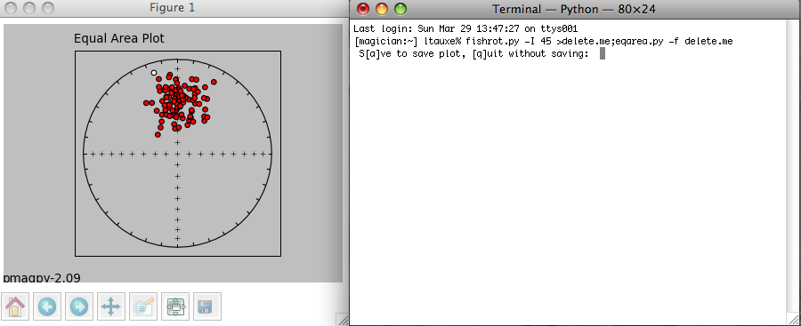
The command fishrot.py creates a fisher distribution with a mean inclination of 45o and saves it in a file called delete.me. eqarea.py makes a plot of it. The tag pmagpy-2.09 in the lower left hand corner is the PmagPy version number that created the plot. You can save the plot in a variety of formats by clicking on the disk icon on the tool bar of the picture (right hand one). Specifying the format name by using the desired suffix in the file name. For example, a file name of myplot.svg would save as an svg format, myplot.png in a png format, etc. The default file format is .svg. Complete details of these and other programs are available through the PmagPy home page.
4.2 Getting Ready for MagIC.py
4.2.1 Setting up a Project Directory
PmagPy uses a number of default file names. While these can be customized by the expert user, it is preferable to keep the MagIC files for a each paleomagnetic study in separate directories. For each study, create a directory with a name that relates to that study. Here we will call it ThisProject. This directory should have NO SPACES in the name and be placed on the hard drive in a place that has NO spaces in the path. Under Windows, this means you should not use your home directory, but create a directory called for example: D:\MyPmagProjects and place ThisProject in that directory.
Inside ThisProject, create two additional directories: MyFiles and MagIC. All the files that you want to import into the MagIC format should be placed in MyFiles and you should just leave MagIC alone unless you really know what you are doing.
Your Directory tree might look like this now:
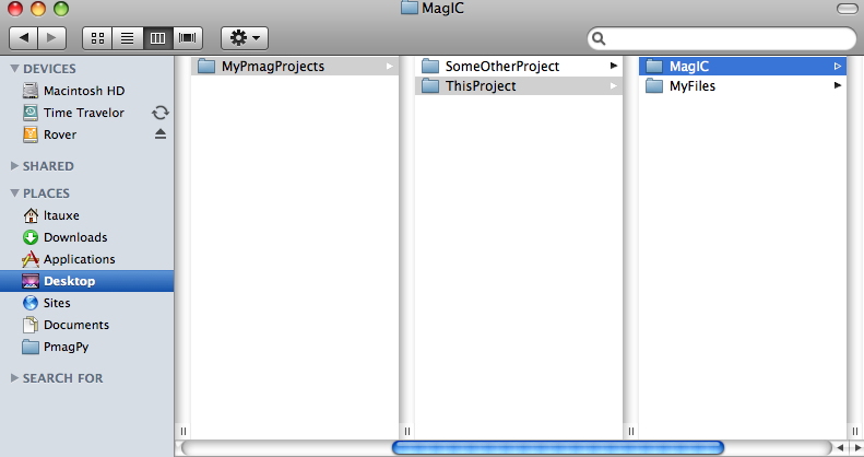
4.2.2 Field Information
Paleomagnetists collect samples in the field and record orientation, location and lithology, etc. in field notebooks. This information is necessary for placing the data into a well characterized context and should be included in the MagIC contribution. Importing field data into the MagIC format using PmagPy requires you to fill in a tab delimited text file with a particular format, here called the "orient.txt" format. These should be placed in the MyFiles directory in the Project directory. When importing the data, you must figure out how your orientation and name schemes relate to what MagIC expects. The process is difficult because there are a multitude of possible naming conventions which relate specimen to sample to site, orientation conventions which convert specimen measurements in geographic and stratigraphic coordinates, etc. PmagPy supports a number of conventions and more can be added by Request. Here we go through each of these problems, starting with the orient.txt file format, and then covering sample orientation and naming schemes.
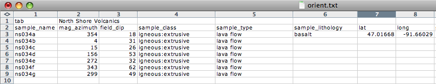
First of all, separate your sampling information into the locations that you plan to designate in the data base. Location name (er_location_name) in MagIC is a rather loosely defined concept which groups together collections of related sites. A location could be for example a region or a stratigraphic section. Location names are useful for retrieving data out of the MagIC database, so choose your location names wisely. Each orient.txt format file contains information for a single location, so fill one out for each of your "locations".
The First Line of the orient.txt file contains two tab delimited fields. The first is the word 'tab' and the second is the location name, in this example it is North Shore Volcanics. Use the same location name EVERY TIME you are asked for it for data related to this collection of samples.
The Second Line of the orient.txt file has the column names. The order of the columns doesn't matter, but the names of the columns do. Some of these are required and others are optional. The example above shows all the REQUIRED fields. Note that latitude and longitude are specified in decimal degrees. mag_azimuth and field_dip are the notebook entries of the sample orientation. Sample class, Lithology and Type are Controlled MagIC Vocabularies, so enter colon delimited lists as appropriate. Also, notice how some fields are only entered once. The PmagPy program (orientation_magic.py) assumes that the last encountered value pertains to all subsequent blank entries.
Optional Fields in orient.txt formatted files are: [date, shadow_angle, hhmm], date, stratigraphic_height, [bedding_dip_direction, bedding_dip], [image_name, image_look, image_photographer], participants, method_codes, site_name, and site_description, GPS_Az
For Sun Compass measurements, supply the shadow_angle, date and time. The date must be in mm/dd/yy format. Be sure you know the offset to Universal Time as you will have to supply that later. Also, only put data from one time zone in a single file. The shadow angle should follow the convention shown in the figure:
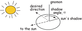
All images, for example outcrop photos are supplied as a separate zip file. image_name is the name of the picture you will import, image_look is the "look direction" and image_photographer is the person who took the picture. This information will be put in a file named er_images.txt and will ultimately be read into the er_image table in the console where addiional information must be entered (keywords, etc.).
Often, paleomagnetists note when a sample orientation is suspect in the field. To indicate that a particular sample may have an uncertainty in its orientation that is greater than about 5o, enter SO-GT5 in the method_codes column and any other special codes pertaining to a particular sample from the method codes table. Other general method codes can be entered later. Note that unlike date and sample_class, the method codes entered in orient.txt pertain only to the sample on the same line.
If there is not a supported relationship between the sample_name and the site_name (see sample naming schemes below), you can enter the site name under site_name for each sample. For example, you could group samples together that should ultimately be averaged together (multiple "sites" that sampled the same field could be grouped under a single "site name" here.
Supported sample orientation schemes:
Samples are oriented in the field with a "field arrow" and measured in the laboratory with a "lab arrow". The lab arrow is the positive X direction of the right handed coordinate system of the specimen measurements. The lab and field arrows may not be the same. In the MagIC database, we require the orientation (azimuth and plunge) of the X direction of the measurements (lab arrow). Here are some popular conventions that convert the field arrow azimuth (mag_azimuth in the orient.txt file) and dip (field_dip in orient.txt) to the azimuth and plunge of the laboratory arrow (sample_azimuth and sample_dip in er_samples.txt). The two angles, mag_azimuth and field_dip are explained below.
[1] Standard Pomeroy convention of azimuth and hade (degrees from vertical down) of the drill direction (field arrow). sample_azimuth = mag_azimuth; sample_dip =-field_dip.
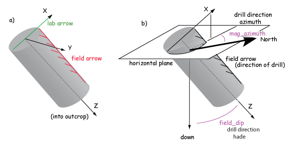
[2] Field arrow is the strike of the plane orthogonal to the drill direction, Field dip is the hade of the drill direction. Lab arrow azimuth = mag_azimuth-90o; Lab arrow dip = -field_dip
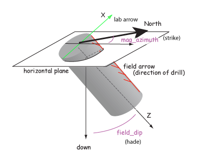
[3] Lab arrow is the same as the drill direction; hade was measured in the field. Lab arrow azimuth = mag_azimuth; Lab arrow dip = 90o-field_dip.
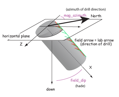
[4] Lab arrow orientation same as mag_azimuth and field_dip.
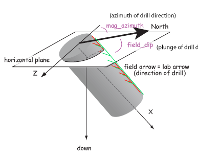
[5] Same as AZDIP convention explained below - azimuth and inclination of the drill direction are mag_azimuth and field_dip; lab arrow is as in [1] above. field arrow are lab arrow azimuth is same as mag_azimuth, Lab arrow dip = field_dip-90o
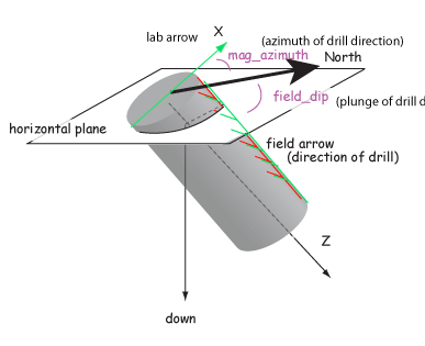
[6] Lab arrow azimuth = mag_azimuth-90o, Lab arrow dip = 90o-field_dip, i.e., field arrow was strike and dip of orthogonal face:
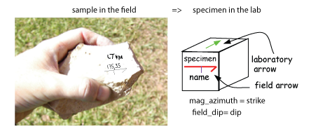
Supported sample naming conventions:
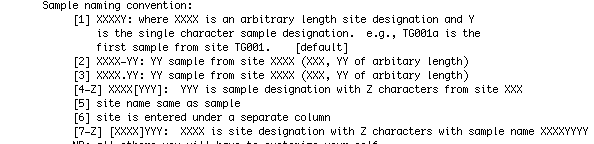
Structural corrections:
Because of the ambiguity of strike and dip, the MagIC database uses the dip direction and dip where dip is positive from 0 => 180. Dips > 90 are overturned beds. Plunging folds and multiple rotations are handled with the pmag_rotations table and are not implemented within PmagPy.
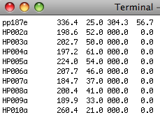
4.2.3 Measurement Data
The MagIC database is designed to accept data from a wide variety of paleomagnetic and rock magnetic experiments. Because of this the magic_measurements table is very complicated. Each measurement only makes sense in the context of what happened to the specimen before measurement and under what conditions the measurement was made (temperature, frequency, applied field, specimen orientation, etc). Also, there are many different kinds of instruments in common use, including rock magnetometers, susceptibility meters, Curie balances, vibrating sample and alternating gradient force magnetometers, and so on. We have made an effort to write translation programs for the most popular instrument and file formats and continue to add new supported formats as the opportunity arises. Here we describe the various supported data types and tell you how to prepare your files for importing. In general, all files for importing should be placed in the MyFiles directory or in subdirectories therein as needed.
Rock magnetometer file formats
Rock Magnetometer File Formats:
Supported files and how to prepare for importing:
CIT format: The CIT format is the standard format used in the paleomagnetics laboratory at CalTech and other related labs. This is the default file format used by the PaleoMag software package. This data format stores demagnetization data for individual specimens in separate sample data files. The format for these is described on the PaleoMag website. The file names with specimen data from a given site are listed in a .SAM file along with other information such as the latitude, longitude, magnetic decliantion, bedding orientation, etc. Details for the format for the .SAM files are located here. Place all the files (sample data files and summary .SAM files) in your MyFiles directory and proceed to the section on MagIC.py.
HUJI format:
The HUJI format is the standard format used in the paleomagnetics laboratory at Hebrew University in Jerusalem.
Under contstruction
LDEO format:
The LDEO format is the standard format used in the paleomagnetics laboratory at Lamont Doherty Earth Observatory and other related labs. Here is an example:
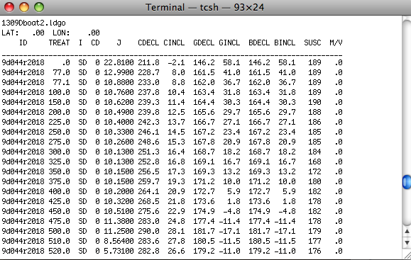
The first line is the file name. The second has the latitude and longitude for the site. The third is a header file with column labels. These are: the specimen name, a treatment key, and instrument code, intensity in 10-4 emu, CDECL and CINCL which the declination and inclination in specimen (core) coordinates. Optionally, there are GDECL, GINCL which are declination and inclination in geographic coordinates, BDECL, BINCL which are in stratigraphic coordinates, SUSC which is susceptibility (in 10-6 SI). Data in this format must be separated by experiment type (alternating field demagnetization, thermal demagnetiztation). Place all data files in your MyFiles directorty and proceed to the section on MagIC.py.
LIV-MW format:
The LIV-MW format is the format used for microwave data in the paleomagnetics laboratory at Liverpool.
Under contstruction
SIO format: The SIO format has six required columns: Specimen_name Treatment_code Uncertainty Intensity Declination Inclination. These are in a space delimited file with no header.
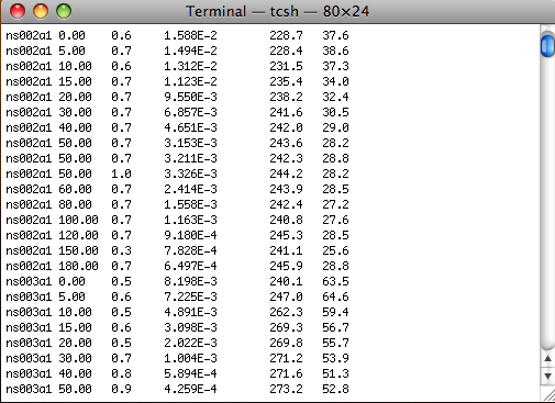
The specimen name is assumed to have a simple relationship to the sample name using characters at the end of the specimen name. All data in a given file must have the same number of characters relating specimen to sample. For example, in the specimen name ns002a1, the terminal number is the specimen number of sample ns002a. If there are many specimens (more than 10, say), one might have a specimen ns002a01, in which case the last two characters are the specimen identifier. All data in a given file must have the same number of characters that serve as the specimen ID. The relationship of the sample name to site name can follow the sample naming convention described in the section on Field Information.
The treatment code specifies the treatment step as well as information about applied fields or even sometimes orientation during treatment (e.g., during an AARM experiment). The treatment code has the form XXX.YYY where YYY is a variable length modifier that can range from zero to three characters in length. For simple demagnetization experiments, the treatment is either the temperature (in Centigrade) to which the specimen was heated and cooled in zero field prior to measurement or the alternating field (in millitesla) to which the specimen was subjected in zero field prior to measurement.
Measurement uncertainty is the circular standard deviation of repeated measurements at the same treatment step (usually in different orientations in the magnetometer.)
Intensity is assumed to be total moment in emu (kAm2).
Declination and inclination are in specimen coordinates.
The optional meta-data string is of the form:
mm/dd/yy;hh:mm;[dC,mT];xx.xx;UNITS;USER;INST;NMEAS
where: hh is in 24 hour, dC or mT units of treatment XXX (see Treatment code above) for thermal or AF respectively, xx.xxx is the DC field, UNITS is the units of the DC field (microT, mT), INST is the nstrument code, number of axes, number of positions (e.g., G34 is 2G, three axes, measured in four positions), and NMEAS is the number of measurements in a single position (1,3,200...).
Treatment codes for special experiments:
XXX.0 first zero field step
XXX.1 first in field step [XXX.0 and XXX.1 can be done in any order]
XXX.2 second in-field step at lower temperature (pTRM check)
XXX.3 second zero-field step after infield (pTRM check step)
XXX.3 MUST be done in this order [XXX.0, (optional XXX.2), XXX.1 XXX.3]
X.00 baseline step (AF in zero bias field - high peak field)
X.1 ARM step (in field step) where X is the step number in the 15 position scheme described here.
XXX.YYY XXX is temperature step of total TRM and YYY is dc field in microtesla.
UB format:
The UB format is the standard format in the University of Barcelona Laboratory and is the 2G binary format. These cannot be viewed with a text editor.
Under construction
UU format:
The UU format is the standard format in the University of Utrecht Fort Hoofddijk Laboratory that is used by the PalMag software package.
Under construction
UCSC format:
Two University of California Santa Cruz formats are supported - the new standard and a legacy file format.
Under construction
2G format: 2G Enterprises ships magnetometers with software that saves data in a binary "2G" format. Each file has the data for a given specimen and must have ".dat" or ".DAT" as a file type (e.g., Id1aa.dat).
PMD (ascii) format:There are two formats called '.PMD': an ascii file format used with the software package of Randy Enkin and a binary format. Both are used with the PaleoMac program written by J.P. Cogne. The ASCII file format is the so-called I.P.G. format described on the PaleoMaC web site. The two different file formats, so be sure you know which one you are using. Here is an example of the ascii (I.P.G., AF) file format:
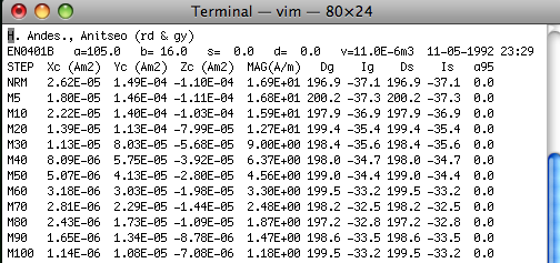
The first line is a comment and the second line has: SPECIMEN a=AZIMUTH b=HADE s= STRIKE d= DIP v=VOLUME DATE TIME. The orientation information AZIMUTH and HADE are of the specimen's 'X' direction (orientation convention #1 in our convention). The third line is a header. The remaining lines are the measurement data. The first column specifies the treatment step: NRM, MXX or TXX. M steps are AF demagnetizing peak fields in mT and T steps are thermal demagnetization temperatures in oC. Columns 2-4 are the X,Y,Z data in specimen coordinates. These are in Am2. Column 5 is the volume normalized magnetization in A/m. Columns 6 and 7 are the Declination and Inclination in geographic coordinates and Columns 8 and 9 are the same in tilt corrected (stratigraphic) coordinates. There are optional columns for alpha95 and susceptibility.
ThellierTool (tdt) format: Here is an example of a TDT formatted file:
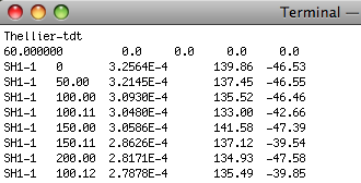
To use this option, place all .tdt files in a directory. You will be asked the usual questions about location, and naming conventions. MagIC.py copies each input file into the MagIC Project directory and generates a command to the program TDT_magic.py which creates a magic_measurements formatted file with the same name, but with a .magic extension. It writes and entry to the measurements.log file so that all the .magic files can be combined when you assemble your measurements. Note that all files in a given directory must have the same location and naming conventions.
Anisotropy of Magnetic Susceptibility File Formats:
.s format: The ".s" option allows strings of data with the format: X11 X22 X33 X12 X23 X13 where the Xii are the tensor elements (remembering that X12=X21, X23=X32 and X13=X31):

There is an optional first column with the specimen name and an optional last column with the standard deviation of the measurements (calculated with the Hext method). Here is an example of a file with the optional specimen name and standard deviation columns:
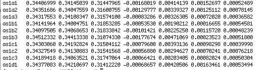
For more on how to measure AMS and calculate tensor elements, see the online textbook chapters of Essentials of Paleomagnetism.
Kly4S format: This data file format is generated by the program described by Gee, J.S., Tauxe, L., Constable, C., AMSSpin: A LabVIEW program for measuring the anisotropy of magnetic susceptibility with the Kappabridge KLY-4S, Geochem. Geophys. Geosyst., 9, Q08Y02, http://dx.doi.org/10.1029/2008GC001976, 2008. It is essentially the same as the .s format (with specimen name in the first column), but has much more information about the frequency, appied field, date and time of measurement, and so on:
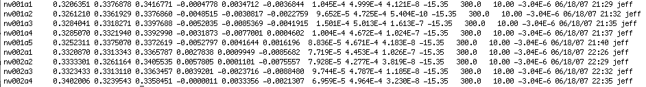
k15 format: The .k15 format has the following format:
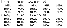
The first row for each specimen contains the specimen name, the azimuth and plunge of the measurement arrow and the strike and dip of the rock unit. The following three lines are the 15 measurement measurement scheme used with the Kappabridge instruments in static mode.
Susar 4.0 ascii format:
This format is generated by the Susar 4.0 program used for running Kappabridge instruments in spinning mode. It is the default program that comes with the instrument. Here is an example of an output file:
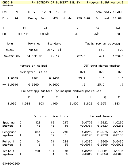
Hysteresis file formats:Hysteresis data can be obtained on a wide variety of instruments from vibrating sample magnetometers (VSM), alternating gradient force magnetic force magnetometers (AGFM), MPMS instruments, etc. As of now, only AGFM data from Micromag instruments are supported and only two of the many possible experiments are supported (basic hysteresis loop and "back-field" curve). These experiments have two different styles of header, the orignal and the "new". Here are some examples:
Basic hysteresis loop:This is an example of the original file format for a "basic" loop".
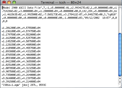
Back-field curve:This is an example of the original file format for a back-field curve.
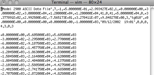
New: Both of these experiments can also be saved with the "new" format. Here is an example of the "new" header:
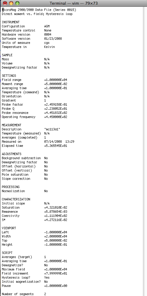
4.3 Using the MagIC.py GUI
The MagIC.py graphical user interface is a Python program that facilitates importing of measurement data and sample information (location, orientation, etc.) into the MagIC format and interpretation thereof. It will help prepare all the files into a text format that can be imported directly into a MagIC smartbook. MagIC.py copies files to be uploaded into a special project MagIC directory, translates them into the MagIC format and keeps track of things in various log files. For this reason, once the project MagIC directory has been created, you should just leave it alone. See the help pages for instructions on setting up the Project directories and installing PmagPy if you have not yet done so. Once you have placed all the needed files (orient.txt formatted files for each location and the measurement data files) in the MyFiles directory, open up a terminal window and type MagIC.py on the command line. Select the MagIC directory in your Project directory when prompted.
If at any time it seems that the MagIC.py GUI is unresponsive or "stuck", click on the Python icon and try again. I think this only happens on Macs, so look on your Dock for the python symbol:

4.3.1 File Menu
Different operating systems will have a different look, but all versions will put up a Welcome window when you have fired up the program MagIC.py. When you pull down the "File" menu, you will see these options:
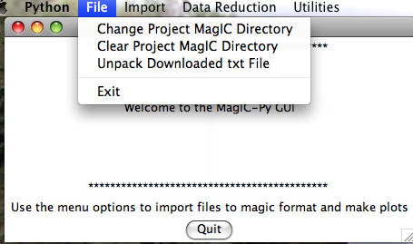
4.3.2 Import Menu
When you pull down the "Import" menu, you will see these options:
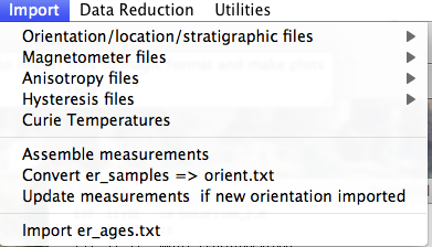
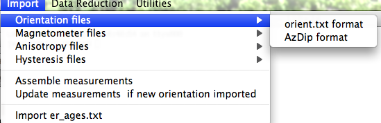

If none fit, then do the transformation yourself and provide the azimuth and plunge of the "X" axes used in your measurements and choose convention #4. Click on the "OK" button to advance to the next window. This will ask you about your preferences for correcting for magnetic declination. The declination used to correct your magnetic compass data will be recorded in the sample_declination_correction field of the er_samples table. If you set your magnetic declination correction to zero in the field and provided the date, latitude and longitude of the sampling location, you can request that orientation_magic.py calculate the declination correction from the (D)IGRF value. It uses the IGRF-10 coefficients which can be downloaded from the National geophysical data center website. Alternatively, you can supply your preferred value on a later page (option 2), or supply magnetic azimuth data that have already been corrected (option 3):
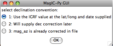
On the next page, you must select your naming convention. Note that for options #4 and 7, the number of characters that distinguish sample from site will be supplied on a later page. If none of these options fit your naming convention, put the site name under the column heading site_name in the orient.txt file. This can also be used to group samples that you wish to average together as a "super-site" mean, assuming that they record the same field state (averaging sets of sequential lava flows, for example.)
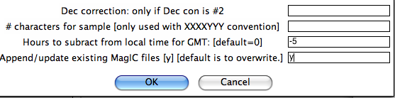
Often a the attitude of the rock units sampled for paleomagnetic study will be oriented multiple times. To average these, one would convert the bedding directions to bedding poles, take a fisher mean of the poles, then convert the mean bedding pole back to dip direction and dip. If you want to do that with the bedding information in the file you are importing, check the box "Take fisher mean of the bedding poles" in this window:
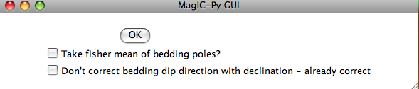
Check the box marked 'Don't correct bedding dip direction with declination....' if you corrected the bedding dip directions for declination already. (It is possible that the bedding dip directions be corrected while the sample orientations are not, for example if the bedding attitudes were read off an existing map...).
The next window allows you to select method codes that describe sample conditions. Select all that apply to all samples. Sample specific method codes can be attached within the orient.txt file itself.
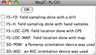
After you get through all the windows, the MagIC.py GUI will generate commands which will appear on your command line prompt. It copies the orient.txt formatted file into the MagIC directory and calls the program orientation_magic.py. This program reads your datafile and parses the information into several MagIC tables (usually er_samples.txt, er_sites.txt, but also er_images.txt if you entered image information in the orient.txt file). If you indicated that you had multiple locations, it will append each subsequent import file to these same filenames. Check the terminal window for errors! If you can't figure out what went wrong, send a screen shot and the offending orient.txt file and I'll try to figure out what went wrong.
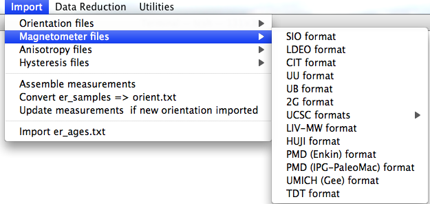
SIO formatted files: In the first window, choose the laboratory protocol from the following menu:
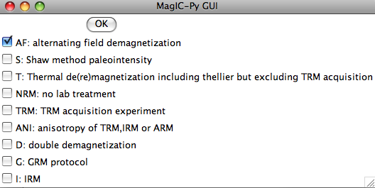
Check all that apply: AF indicates that the data are from an alternating field demagnetization experiment. If a double or tiriple (GRM) demagnetization protocol was followed, also check the D and G boxes. For thermal demagnetization and also double heating paleointensity experiments, check the 'T' box. Do not check this box, however, if the data are from a TRM aquisition experiment (multiple field steps with total TRMs). If these data are some form of anisotropy experiment, check the ANI box and if they are IRM data, check the IRM box.
Enter a variety of important information in the next window:
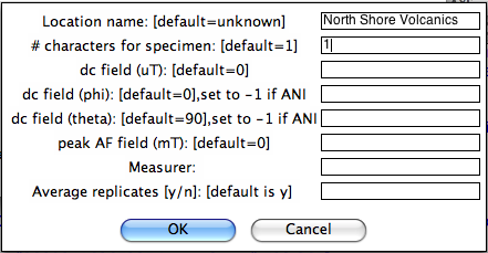
Now you must choose your naming convention. NB: All specimens must have the same naming convention within a single file. After collecting all the required information, MagIC.py generates a call to the program mag_magic.py which sorts the measurement data out into the MagIC format. Each imported file is stored as a file of the same name as the input file, but with .magic appended to the end. Check the terminal window for errors. It will also let you know about all the averaging that has taken place - these comments are not errors. After all the measurement files have been imported, select "Assemble measurements" from the Import pull down window. You are now ready for "Data reduction".
Other formats:
LDEO format:
CIT format:
UU format:
UB format:
2G format: To use this option, first place all the 2G binary .dat files in a separate sub-directory within your MyFiles directory. All the files in a given sub-directory must have the naming convention, sampling meta-data and location name. You will first be asked to specify the directory to import and then the naming convention (see instructions for .PMD files below). Be sure to assemble your measurements before attempting to make plots from them.
UCSC format:
LIV-MW format:
HUJI format:
PMD (ascii) format: To use this option, first place all the .PMD formatted file in a separate sub-directory within your MyFiles directory. All the files in a given directory must have the same naming convention, sampling meta-data and location name. You will first be asked to specify the directory to import:
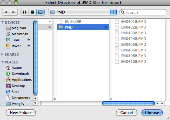
Then you will be asked to specify the naming convention that you have used. Additional information can be supplied in the table:
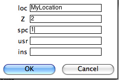
Notice that because if you specified naming conventions #4 or #7. (e.g., specimen EN0401B is from sample EN0401 and from site EN04), we must supply the number of characters designating sample from site here (2), as well as the number of characters designating specimen from sample (1). We can specify some of the sampling conventions using the magic method codes on this page:
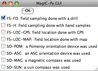
Normally, you should elect to average replicate measurements at a given treatment step, but some studies you may not want to, so you are given the option here:
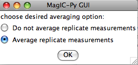
If you have already imported orientation information and created a file called er_samples.txt, the program will ask you if you want to append this information to that file (updating any existing sample orientation information in the process) or to create a new file, overwriting all existing information. This option allows you to keep .PMD files from separate locations in different directories, uploading them separately and combining all the information together into your er_samples.txt and magic_measurements.txt files. When you are finished uploading measurement data, select the Assemble Measurements option so that you can plot the data.
PMD (IPG-PaleoMac) format: You will first be asked to specify the import file, then you will be asked to specify the naming convention that you have used. Additional information can be supplied in the table:
Normally, you should elect to average replicate measurements at a given treatment step, but some studies you may not want to, so you are given the option here:
If you have already imported orientation information and created a file called er_samples.txt, the program will ask you if you want to append this information to that file (updating any existing sample orientation information in the process) or to create a new file, overwriting all existing information. This option allows you to keep files from separate locations in different directories, uploading them separately and combining all the information together into your er_samples.txt and magic_measurements.txt files. When you are finished uploading measurement data, select the Assemble Measurements option so that you can plot the data.
TDT (ThellierTool) format: This option allows input of the ThellierTool format for double heating experiments. You will be asked all the usual questions regarding the directory in which the .tdt files reside, the naming convention, and the location name. Be sure that each directory contains files with the same location and naming conventions. MagIC.py will copy each file into the MagIC Project directory and generate a command to the program TDT_magic.py which does the conversion to a magic formatted measurement file. When you are finished, select "Assembls Measurements" and proceed to viewing of Thellier data under the "Data Reduction" menu.
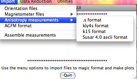
All options generate commands, depending on the file type, which create MagIC formatted files, in particular the rmag_anisotropy.txt format file which is used by the plotting programs for AMS (see Data reduction).
.s format: This option imports .s formatted files. After choosing the file for import, the GUI will allow you to specify if you have the specimen name in the first column and a sigma value in the last:
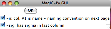
KLY4s format: This option imports KLY4s formatted files. These files are essentially enhanced .s files and this option has enhanced features. If you have imported orientation information it will do the transformations from specimen to geographic and stratigraphic reference frames which can then be plotted with the anisotropy plotting options. If you have not imported orientation information, the program will complain, but go ahead with the importation - note that the other reference frames will not be available until you re-import the KLY4s file. You will be asked to specify your naming convention and supplemental information:
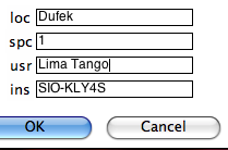
Type in your "location" on the line labeled 'loc', the number of characters used to differentiate between specimen and sample, who made the measurements (optional) and on what instrument (optional) in the "usr" and "ins" lines. The GUI first copies your data file into the MagIC project directory and then constructs a call to kly4s_magic.py on the command line. Check the terminal window for errors! Be sure to "assemble measurements" before attempting to plot your data.
K15 format: This option imports K15 formatted files. These files have the orientation information embedded in them. If you have not already imported orientation information for a particular sample, the embedded information will be added to the existing er_samples.txt file. If none exists, a new er_samples.txt file will be created. You will be asked to specify your naming convention and usual supplemental information. Type in your "location" on the line labeled 'loc', the number of characters used to differentiate between specimen and sample, who made the measurements (optional) and on what instrument (optional) in the "usr" and "ins" lines. The GUI first copies your data file into the MagIC project directory and then constructs a call to k15_magic.py on the command line. Check the terminal window for errors! Be sure to "assemble measurements" before attempting to plot your data.
SUSAR ascii format: This option imports SUSAR ascii formatted files. These files have the orientation information embedded in them. If you have not already imported orientation information for a particular sample, the embedded information will be added to the existing er_samples.txt file. If none exists, a new er_samples.txt file will be created. You will be asked to specify your naming convention and usual supplemental information. Type in your "location" on the line labeled 'loc', the number of characters used to differentiate between specimen and sample, who made the measurements (optional) and on what instrument (optional) in the "usr" and "ins" lines. The GUI first copies your data file into the MagIC project directory and then constructs a call to k15_magic.py on the command line. Check the terminal window for errors! Be sure to "assemble measurements" before attempting to plot your data.
When you expand the "Hysteresis files" menu, you are presented with several choices:
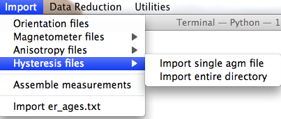
Import single agm file: This option constructs a call to the agm_magic.py program. You will first be asked to select the file for importing. This file can be in either the old or the new format - the program can figure out which automatically. Then the program requests that you select the most appropriate naming convention. These relate sample names to site and location names. The first five options are useful if there is a simple relation ship between sample and site names and all the files come from a single location. Option #6 allows you to have more complicated relationships between samples, sites and location names by specifying these "by hand" in an er_samples.txt file in your MagIC project directory. If you imported orientation information using an orient.txt file, by specifying the site name for each sample under a column labeled site_name, and importing multiple orient.txt formatted files for the individual locations involved in the study, your er_samples.txt file will already be available to you for this option. The final option is for "synthetic" specimens. Choose this if there is no "site" or "location" information and the sample is only of rock magnetic interest. Next you will be asked for additional information, for example, location name, number of characters that distinguish specimen from sample, the specimen name, etc.
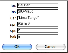
Check your terminal window for specific definitions. Note that agm_magic.py assumes that the input file name had the specimen name as the root, but you can change the specimen name on the line labelled 'spn'. In this example there are two characters that distinguish the specimen (IS01a-1) from the sample (IS01a) and the naming convention was #1 (IS01a is a sample from site IS01). The program copies your data file into the MagIC project directory and calls agm_magic.py with switches set by answers to the queries set by the GUI. The actions can be viewed in your terminal window. agm_magic.py will create an output file with the same name as your input file, but with the .magic extention and write this file name to the measurements.log file. Note that if this is a "backfield" IRM experiment, you should type 'y' into the data entry window on the line labelled 'bak'.
Import entire directory: This option is very similar to the "single agm file" option described above - but allows automatic import of all files within a specified directory. The differences are that all files must have the specimen name as the file name root, and they must all have the same naming convention as you will only be asked once for all the information.
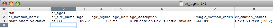
It is very important that you attach the proper method codes to your age information, so check the "Geochronology Methods" options carefully. Also, you will want to include the proper references in the er_citation_names field. You can add the citation information within the MagIC Console after your data get imported into it. To import the age file into the MagIC project directory, place the er_ages.txt file in your MyFiles directory and select the "import er_ages.txt" option in the Import menu.
4.3.3 Data Reduction Menu
When you pull down the "Data reduction" menu, you will see these options:
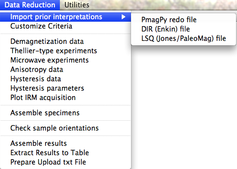
The zeq_redo file contains instructions for how to interpret measurement data for a standard demagnetization experiment. The first column is the specimen name, the second is the directional estimation method codes (DE-BFL for best-fit lines, DE-BFP for best-fit planes and DE-FM for Fisher means). The third column is the beginning demagnetization step for the calculation and the fourth is the end. Please note that these must be in the units required by the MagIC database, so are tesla for AF demagnetization and kelvin for thermal demagnetization. All magnetometer data are translated into these units. To convert mT to tesla, multiply by 10-3, Oe to tesla, multiply by 10-4 and from degrees C to kelvin, add 273. The fifth column is an optional component name. If none are supplied, the first interpretation for a given specimen is named "A" and the second is named "B", etc.
The thellier_redo file contains instructions for how to interpret measurement data for a double heating paleointensity experiment. The first column is the specimen name, the second is the beginning demagnetization step for the calculation and the third is the ending demagnetization step. Units must be in oC. To convert from degrees C to kelvin, add 273.
When you select the "PmagPy redo" option, the MagIC.py GUI copies the redo file into your project MagIC directory and executes the commands zeq_magic_redo.py or thellier_magic_redo.py, depending on what you imported. This program hunts through measurement data (in the magic_measurements.txt file) for data matching each specimen name, collects the data between the two end points specified in the redo file and does the desired calculation. The specimen calculations are written to a pmag_specimen formatted file called either zeq_specimens.txt or thellier_specimens.txt within your project MagIC directory. These interpretations will be read in when you try the Demagnetization data or Thellier-type experiments as described below.
The DIR (ASCII) format is a file format used by the PaleoMac program developed at IPG by J.-P. Cogne. Here is an example of the ASCII version of these files:
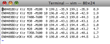
The meanings of the various columns is described on the PaleoMac website. This option copies the selected file to the MagIC project directory and generates a call to the program DIR_magic.py. This translates the file into a zeq_redo formatted file (see above) called DIR_redo. It then called zeq_magic_redo.py to make a file called zeq_specimens_DIR with the MagIC formatted specimen directions in it. Note: this will overwrite any "DIR_redo" file already imported, so put ALL your interpretations into a single .DIR file! To assemble different specimen direction files together, choose "Assemble Specimens" as described below.
The LSQ format imports the interpretions stored in the .LSQ files output by the Craig Jones program PaleoMag and described on this website. Here is an example of the data format:
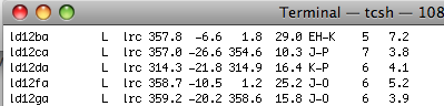
To use this option efficiently concatenate all the .LSQ files from a particular study into a single .LSQ file. You can do this by typing the command: cat *.LSQ >myLSQ on your command line if you are in the directory in which all the .LSQ files are located. Alternatively, you can import each .LSQ file individually. On choosing this option, you are asked to specify the file name to be imported and then whether or not you want to overwrite your previous specimen interpreation files. If you are importing all the interprations in a single .LSQ file (recommended), you should select the "overwrite" radio button. If you don't, you will generate a file called zeq_specimens_LSQ.txt which you can select when assembling your results.
The LSQ option first copies the .LSQ file into your MagIC project directory, then calls the program LSQ_redo.py. This program does two things: it creates a zeq_redo formatted file (see above) and it modifies the magic_measurements.txt file to mark the sample_flag to 'b' for bad for the excluded data points as indicated in the .LSQ file. Then the MagIC GUI generates pmag_specimen formatted file. You then should select "assemble specimens" and check your interpretations using the "Demagnetization Data" plotting option described below.
The first window allows you to specify what sort of criteria file you want to create:
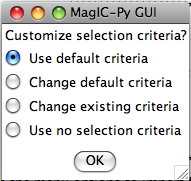
You can either use the default criteria or change them to suit your own needs. You can modify a criteria file you created before or apply no selection criteria. For changing default of existing criteria, you will then be asked to customize a series of criteria. The first is for choosing directional data for specimens:
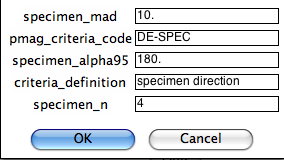
Next you can select criteria for intensity data at the specimen level:
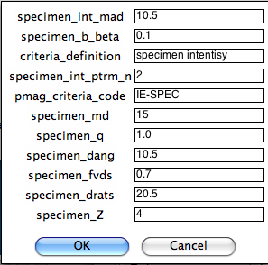
Next you can select criteria for directional data at the sample level (based on averages of multiple specimens:
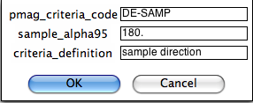
Next you can select criteria for directional data at the sample level (based on averages of multiple specimens:
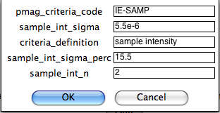
On the next page, you can customize the same parameters but for the site level:
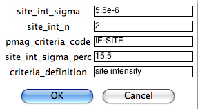
Here you customize your criteria for site level directions:
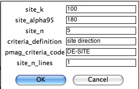
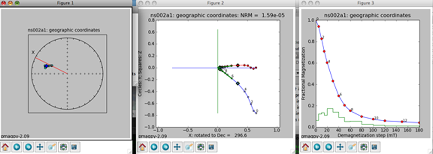
The left-hand plot is an equal area projection of the demagnetization data. The title is the specimen name and the coordinate system of the plot. Solid symbols are lower hemisphere projections. The directions of lines fit through the data are shown as blue diamonds. Green dotted lines (not shown) are the lower hemisphere projections of a best-fit plane while cyan is on the upper hemisphere. The red line is the X direction (NRM) of the middle plot.
The middle plot is a vector-end point diagram. The magnetization vectors are broken down into X,Y,Z components (depending on the coordinate system). The default for this plot is to rotate the X direction such that it is parallel to the NRM direction. Solid symbols are the horizontal projection (X,Y) and open symbols are the X,Z pairs - the plane containing X,Z is shown as the solid red line in the left-hand plot. The open diamonds are the end points for the calculations of any components from prior interpretations. Green lines are best-fit lines. The numbers are the demagnetization steps shown in the terminal window. The title is the specimen name, the coordinate system and the NRM intensity (in the units of the magic_measurements table, so are SI.
the right-hand plot is the behavior of the intensity during demagnetization. Numbers are the demagnetization steps listed in the terminal window. The green line is the magnetization lost at each step.
You control the program through the terminal window:
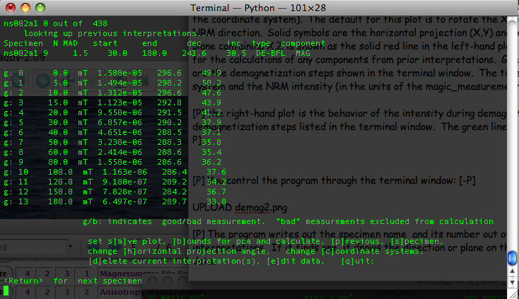
The program writes out the specimen name and its number out of the total, then looks for previous interpretations. If it finds one, it draws the direction or plane on the plot windows and prints out summary data: the specimen name, the number of steps included in the calculation, the MAD or alpha_95 (depending on calculation type), the start and end demagnetization steps, the declination and inclination of the directed line or pole to the best-fit plane, the calculation type (best-fit line, plane or fisher mean or DE-BFL, DE-BFP, DE-FM respectively) and the component name.).
Then, the program prints out the data for the specimen. Each measurement is annotated "g" for good or "b" for bad depending on the measurement_flag in the data file and numbered. The demagnetization level is given in mT or oC. The strength is in SI units and the declination and inclination are in the coordinate system specified in the titles of the plot figures.
The program can be controlled by entering letters on the command line. Hitting the return (or enter) key will step to the next specimen.
When you have stepped through all the specimens, or typed 'q' to quit, the program quits and control is returned to the GUI window. If it seems stuck, click on the python icon on your dock (Macs only) and the GUI will respond again (usually!).
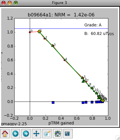
The left-hand plot (labeled Figure 3) is an Arai plot of the double heating experiment. The title is the specimen name and NRM intensity of the specimen. Solid symbols are zero-field first then in-field heating pairs (ZI) data and open symbols are in-field first, then zero field pairs (IZ). The temperature pairs are numbered for reference with the data list in the terminal window. The blue squares are "pTRM-tail checks" and the triangles are "pTRM" checks. If you have selected end points for inclusions in the slope calculation, these will be marked by diamonds and the green line is the best-fit line through the data points. The field intensity will be noted (B: ) in microtesla and a grade assigned according to the selection criteria. To change these, use the "customize criteria" option described above. The line labeled "VDS" is the vector difference sum of the zero field data.
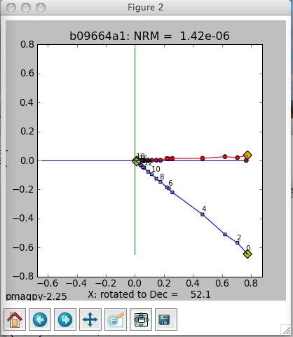
The middle plot is a vector-end point diagram. The magnetization vectors are broken down into X,Y,Z components (these are in specimen coordinates here with the X direction rotated such that it is parallel to the NRM direction. Solid symbols are the horizontal projection (X,Y) and open symbols are the X,Z pairs. The open diamonds are the end points for the calculations of any components from prior interpretations. Green lines are best-fit lines. The numbers are the demagnetization steps shown in the terminal window. The title is the specimen name and the NRM intensity (in the units of the magic_measurements table, so are SI.
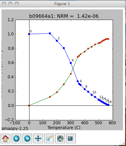
The right-hand plot is the behavior of the intensity during demagnetization and remagnetization. Numbers are the demagnetization steps listed in the terminal window.
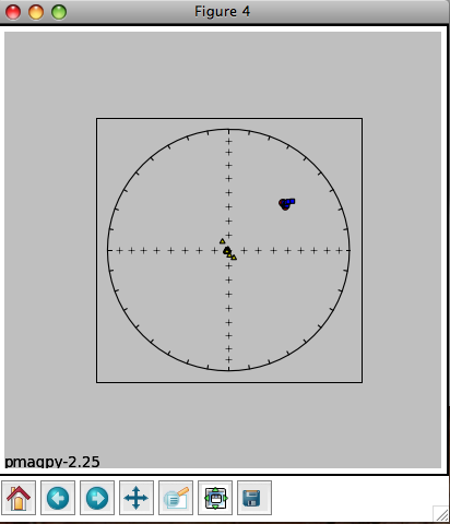
The fourth plot is an equal area projection of the zero field steps from the ZI steps (circles) and the IZ steps (squares) as well as the direction of the pTRM acquired at each step (triangles). This should of course be parallel to the lab field direction and deviation therefrom is a hint that the specimen is anisotropic. Only the steps included in the slope calculation are plotted.
You control the program through the terminal window:
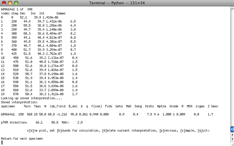
The program writes out the specimen name and its number out of the total, then looks for previous interpretations. If it finds one, it draws the interpretations on the plot windows and prints out summary data: specimen name, lower and upper temperature steps (Tmin, Tmax), the number of steps used in the calculation, N, the lab field assumed, lab_field, the ancient field estimate (no corrections) B_anc and a host of other statistics: b q f(coe) Fvds beta MAD Dang Drats Nptrm Grade R MD% sigma Z Gmax which are described in the Essentials of Paleomagnetism online text book. The program also looks for TRM acquisition data and anisotropy data. If it finds it, it will print out the "corrected data" as well, including the corrected pTRM acquisition steps - a proper anisotropy correction will bring the best-fit line through these into alignment with the laboratory applied field direction. If the program finds TRM aquisition data, there will be a fifth plot, showing these data as well and the correction inferred therefrom.
The program thellier_magic.py can be controlled by entering letters on the command line. Hitting the return (or enter) key will step to the next specimen.
When you have stepped through all the specimens, or typed 'q' to quit, the program quits and control is returned to the GUI window. If it seems stuck, click on the python icon on your dock (Macs only) and the GUI will respond again (usually!). When you are done, be sure to select "Assemble specimens."
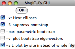
For a complete discussion of confidence ellipses see Chapter 13 in the Web Edition of the book Essentials of Paleomagnetism, by Tauxe et al. (2009). In this example, we elected to plot both the Hext ellipses and the bootstrap ellipses. To suppress the latter, check the box labelled '-B' in the options window. For now, we get this plot:
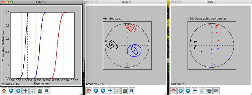
In Figure 1 (to the right), we have plotted the eigenvectors from site tr24. Red squares are the eigenvectors associated with the maximum eigenvalues for each specimen. Blue triangles are the intermediate and black circles are the minima. All plots are lower hemisphere equal area plots. Figure 2 (middle) shows the two forms of confidence ellipses. The rounder, larger ellipses are the Hext ellipses. Green lines are plotted on the upper hemisphere. Figure 3 (left) shows cumulative distributions of bootstrapped eigenvalues and their 95% confidence bounds (vertical lines). Because each eigenvalue is distinct from the others (the confidence bounds do not overlap), this site has a triaxial fabric. These plots can be saved in a variety of formats by clicking on the disk icons to on the figure tool bars by choosing the appropriate name (e.g., myfig.png saves the file in the png format) or by typing an "a" on the command line in the terminal window. [P] [P] To control the program, type in commands on the command line in your terminal window:
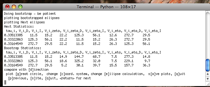
You can change coordinate systems (if you have imported orientation information along with your anisotropy files) by typing a "c", ellipses style, by typing an "e". You can also plot a direction (a lineation observed in the outcrop) or a great circle (the plane of a dike) for comparison. You can also step forward to the next site or back to the previous one. The summary statistics for each ellipse calculation are also printed out in the terminal window. The tau_i are the eigenvalues and the V_i are the eigenvectors. The D's and I's are declinations and inclinations and the zeta and eta are the semi-axes of the major and minor ellipses respectively. These summary statistics calculated by aniso_magic.py are also stored in the file rmag_results.txt in the project MagIC directory.
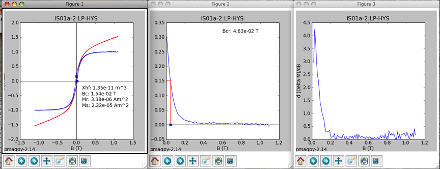
If you also imported data from "back-field" IRM experiments, you will also see a plot like this:
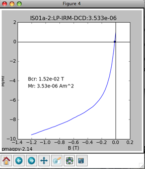
The point at which the remanence is reduced to zero is another estimate for coercivity of remanence. The various hysteresis parameters that are calculated by hysteresis_magic.py are stored in the datafiles rmag_hysteresis and rmag_remanence in the project MagIC directory.
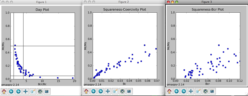
Then, the program steps through the data by site, plotting all the directions in geographic coordinates.
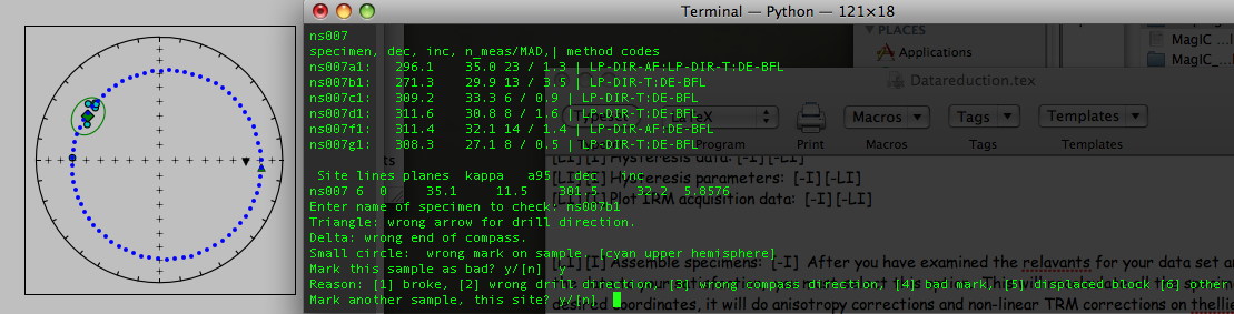
If you find a site with a suspicious sample, you can select 'e' and type in that specimen name on the command line. The program calculates possible specimen directions assuming several common types of errors in the field. Triangle: wrong arrow for drill direction, e.g., out of the outcrop instead of in. Delta: someone read the wrong end of compass. Small circle: wrong mark on sample [cyan upper hemisphere]. Paleomagnetitsts often mark the sample orientation with a brass rod, then extract the sample with a "shoe horn" of some sort. It is possible that when marking the sample, a stray mark was used. In this case, the "real" specimen direction will lie along the dotted line. If any of these possibilities brings the specimen direction into the group of other directions, you can mark this sample orientation as "bad" with a note as to why you have excluded it. The data do not disappear from the data base, but your rationale for excluding a particular result is explained in the er_samples table. The result can be excluded from site means, etc.
When you are done with editing sample orientations, be sure to select "Assemble specimens" again. This will recalculate the specimen tables, excluding the "bad" orientation data from geographic and tilt corrected records.
Then you are asked which (of the possibly many) specimen files you wish to work on. The default is the pmag_specimens.txt file generated by the "Assemble specimens" option. If for example, you only want to work on a particular one, select "customize choice". Usually you will want the default specimen file.
The next window allows you to control which data are selected and how they are treated. To use the selection criteria chosen by you in the "Customize Criteria" section, check the box marked '-exc'. -aD and -aI do the averages by sample, then by site instead of treating all specimens as individuals at the site level. -sam puts sample level VGPs and/or V[A]DMs on the results table. -p plots directions by site so you can have a last check on what is going into the er_sites and pmag_results tables. Virtual Axial Dipole moments (VADM) require an estimate of paleolatitude. This could be the present latitude (-lat option) or a reconstructed paleolatitude (-fla). For the latter, you will have to enter the site name and your best estimate for paleolatitude in a separate file (model_lat.txt). This file should be copied into the project MagIC directory. This latitude will be saved as the model_lat on the results table. If you want to calculate paleolatitudes for a given site, use the "Expected directions/paleolatitudes" option under the Utilities menu. By skipping directions or intensities if you have no relevant data, you can speed up processing time.
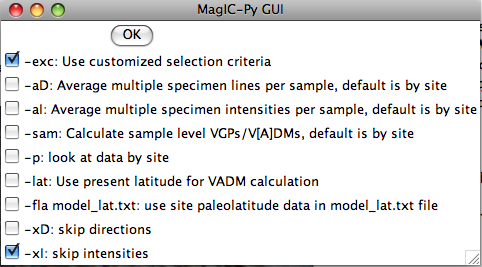
If you have multiple coordinate systems available (e.g., specimen, geographic, tilt corrected), you can choose which coordinate systems you want to include on the pmag_results table:
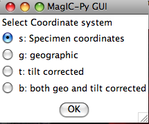
The specimens_results_magic.py program processes the data, averaging by sample (if desired) and by site. It combines best-fit lines and planes at the site level using the technique of McFadden and McElhinny (1988) and calculates VGPs and V[A]DMs as approprite and creates the files pmag_samples.txt, pmag_sites.txt and pmag_results.txt in the project MagIC directory.
4.3.4 Utilities Menu
When you pull down the "Utilities" menu, you will see these options:
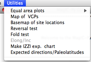
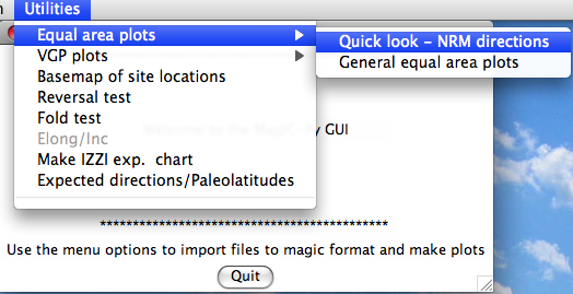
Choosing the "Quick look" option will cause the program to search through the magic_measurements.txt file in your project MagIC directory. The MagIC.py GUI will look into a file called coordinates.txt which is created when you import an orientation file. If you haven't you will only be able to look at the data in specimen coordinates. If you have, you will be asked to specify which coordinate system you desire. Click on the one you want, then on the 'OK' button. You will then see a plot something like this:
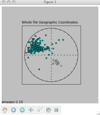
The title will specify the coordinate systems. As usual, solid symbols are lower hemisphere projections. In the terminal window, you will see a list of all the specimens that were plotted along with the "method of orientation (SO-) and the declination and inclination found. You can save the plot in the default format (svg) or in some other supported format (e.g., jpg, gif, png, eps) by clicking on the save (the little diskette icon) button on the plot. The default file format can be imported into for example Adobe Illustrator and edited.
Choosing the general option allows more possibilities, depending on what you have done. You must have selected Assemble Specimens to plot specimen directions or great circles. To plot data for sample or site means, you must first Assemble results. Assuming you have done both, you will be presented with a window that looks something like this:
Choose the level you desire by clicking on it, then click on the "OK" button. Next, you must choose which level you want to plot. Be aware that you could choose to plot at the specimen level yet have chosen to look at the site table which has no specimen level data. In that case you would get a message that there were no data to plot. Here we choose to plot the whole file:
Now you can choose what sort of confidence ellipse you want to plot. Fisher statistics, including how to combined lines and planes are explained in Chapter 11 of Tauxe et al., 2009 and the other methods are explained in Chapter 12. Select the method of choice (or None) and click on the "OK" button.
Finally, select your desired coordinate system. You will be presented with a list of options based on what you imported as orientation information. However, if, for example, when you prepared the results file you choose only the geographic coordinate system and not the tilt corrected one, choosing the tilt corrected coordinate system here will result in no data to plot. Here we chose the geographic coordinate system and were presented with this plot:
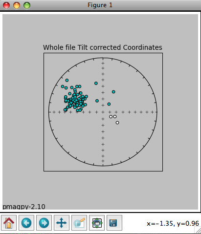
The title reflects the choices that were made. The plot can be saved using the save button or on the command line. In the terminal window you will see a list of the data that were plotted, and the associated method codes. When the eqarea_magic.py program is finished, control will be returned to the MagIC.py
If you choose a coordinate system that is not in the pmag_results.txt file (either because there were no orientation data imported or you did not choose to include it when you assemble the results table), you will have no data to plot. Then you will be asked if you want to flip reverse data to their antipodes. In fact, this option takes all negative latitudes as reverse, so you should be careful with data sets from the Paleozoic or PreCambrian:
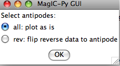
You can customize the projection by setting the position of the "eye". The default is a polar projection.
You will get a plot something like this:
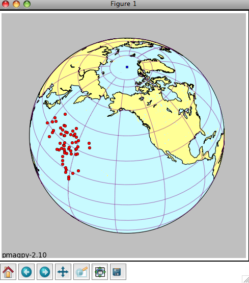
The green square is the spin axis. If you elected to flip 'reverse' data, they will be plotted as green triangles. The plot can be saved in the default format (svg) by typing 'a' on the command line followed by a return (enter) key. For other formats, use the save button on the plot window.
Depending on your choices, you may get a plot like this:
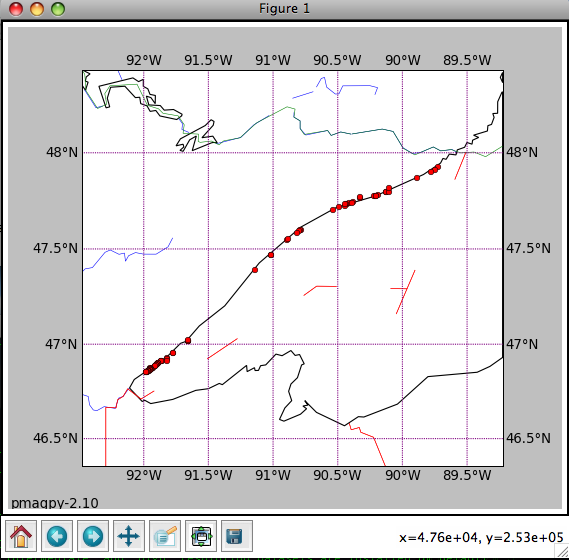
Save the plot by typing 'a' on the command line followed by a return (enter) key, or using the save file button on the plot window itself.
Then it will ask about selection criteria:
And finally, it will give a plot similar to this:
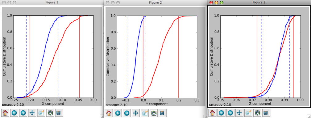
The program takes your data and breaks it into two modes: normal and reverse. It flips the directions in the second mode (usually the reverse one) to their antipodes. Then the program computes the mean direction for each mode and computes the X, Y and Z components for these means directions. Then it re-samples the dataset randomly (a bootstrap pseudo-sample with replacement), generating a new data set which it breaks into two modes, and calculates the components of the mean directions of these. This it repeats 500 times, collecting the components of the two modes. When the bootstrap is finished, the three components of the two modes are sorted and plotted as cumulative distributions in the three plots with the two colors (red for the first mode and blue for the second). The bounds containing 95% of the values get plotted as vertical lines for the two modes. A negative reversals test is achieved when the bounds for the two modes for any of the three components exclude each other.
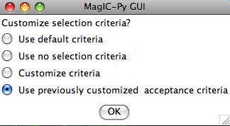
Then the program will generate plots like these:
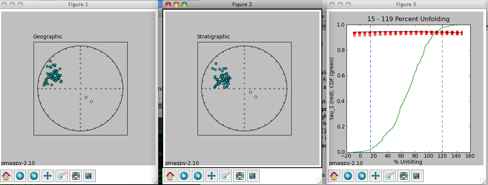
The left hand plot is of the data in geographic coordinates, the middle is after 100% tilt correction and the right hand plot is a cumulative distribution plot of the maximum eigenvalues obtained through principal component analysis of bootstrapped data after various percentages of untilting. This is a measure of concentration that does not require sorting data out by polarity. The vertical bars are the limits bounding 95% of the data. This particular result is not very impressive allowing peaks in concentration spanning virtually the whole range. The dashed red lines represent the behavior of 20 (out of 1000) bootstrapped data sets.
4.4 Tutorial
4.4.1 Directional Study
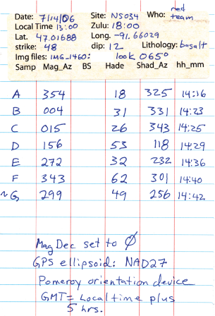
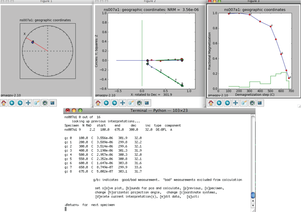
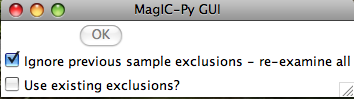
The check orientation option calls the program site_edit.py and steps through the data site by site, printing out sample/specimen information in the terminal window and plotting them, along with the Fisher mean and alpha_95 in the picture window. If a particular directions looks out of place, e.g., ns007b1 in the example data set shown here,
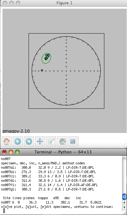
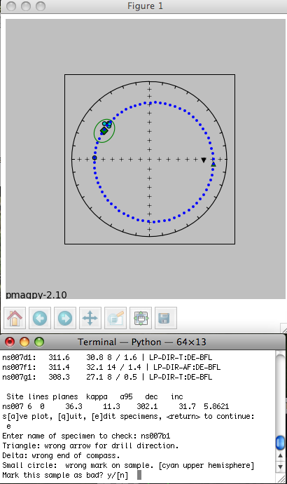
The blue dotted line traces the directions that would be generated if a stray mark on the sample was used instead of the actual drill direction - an interpretation which seems reasonable because the blue dotted line goes right through the directions from all the other specimens at the site. Therefore, type in a 'y' on the command line. And choose "bad mark" as the explanation for rejecting this sample's data. This will mark the sample_flag in the er_samples.txt file as "b" and write in the reason under the sample_description field. Stepping through all the sites allows you to throw out clearly mis-oriented data from your interpretations while preserving the data and the rationale in the database. When the program site_edit.py has finished. You will be asked to run "Assemble Specimens" which is a necessary step before you "Assemble Results". So be sure to choose "Assemble Specimens" from the Import menu before proceeding.
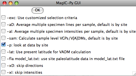
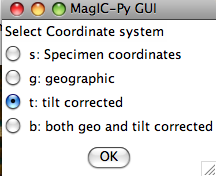
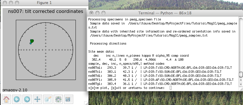
The magic_method_codes summarize how each specimen was treated. The "LP-DIR" method code tells you what type of demagnetization experiment was done (T for thermal, AF for alternating field), the "SO" code tells you about sample orientaion (sun or magnetic compass, for example), the "DE" code documents how the direction estimation was done (BFL for best-fit line or BFP for best-fit plane, for example), the "DA" code lists data adjustments (DIR-GEO, means the data were transformed to geographic coordinates and DIR-TILT means they were also adjusted for tilt). If there is a problem with a site, you can quit the program and return to demagnetization data, or any previous step to track down and fix any problems. If you are satisfied, just step through the sites (there is only one for this tutorial) and the program will finish.
4.4.2 Rock Magnetic Study
Under construction
5 MagIC Glossary
In this Glossary you will find definitions for common nomenclature as used inthe MagIC Website and MagIC Console Software. This section has been added so to make data entry and searching in the database more transparent.
5.1 Terminology and Definitions
Criteria Codes can be defined in the PMAG_criteria and RMAG_criteria tables, and describe on what basis you have been selected or deselected data in your calculations. Once you have defined your Criteria Codes you can assign them to the appropriate data records in your MagIC SmartBooks.
An Expedition is defined either as a land expedition, a seagoing cruise or a fieldwork.
An Experiment Name is a unique identifier for a particular experiment you carried out in your laboratory on a particular specimen or synthetic material. It is recommended that you keep these Experiment Names short and unique. For example, you could device a naming scheme that combines your Institution Name, the Instrument you measured on, the Year of the measurements, and a Unique Enumerator. This would result in Experiment Names like SIO-06-00001 or IRM-X106-0456 that you can use in your publications while allowing others to uniquely refer to your particular experiments.
Even though uncommon in paleomagnetic and rock magnetism, you can provide Fossil information in the MagIC Database. Only provide this information in the MagIC Database when the measurements were carried out on single fossils, pieces of macrofossils or fossil separates. Note that er_fossil_name inside the MagIC SmartBooks refers to a sample number, not its classification.
A Location is defined as any locality that may contain a collection of sites that have been studied. These may include land (stratigraphic) sections, camps or villages for archeological studies, drill cores in lakes, and drill sites for DSDP, ODP and IODP expeditions. Most times Locations fall in a constricted latitude-longitude box, other times they span a larger area. It is, however, advisable to define Locations as narrow as possible, to make them more unique in the database and thus more valuable (i.e. accurate) in searches.
The MagIC Console Software has been developed to help you enter data in the MagIC SmartBook files, to help you check for correctness and coherence in data entries, and to help you prepare these data files for uploading in the online MagIC Database.
The MagIC Database is a relational Oracle 10x database that is located and maintained at the San Diego Supercomputer Center (SDSC) in San Diego, California. This database is an integral part to the EarthRef.org Database and Website and contains both paleomagnetic and rock magnetic data, ranging from measurement data to highly derived magnetic parameters. The database is accessible through the EarthRef.org website and the specific PMAG and RMAG web portals.
A typical MagIC SmartBook file contains 30 tables (or worksheets) in a Microsoft Excel© workbook compliant with the Standard Data and Metadata Format vX.X as defined by the international MagIC consortium. For each project (or publication) a single MagIC SmartBook file should be populated with paleomagnetic and rock magnetic data. When populated, these filled-in SmartBooks can be uploaded into the MagIC Database via an online upload wizard.
Method Codes are short (unique) acronyms or abbreviations that describe a certain method, lab protocol, treatment step, etc. They were devised to allow you to uniquely (and fully) describe the analytical details of your measurement by concatenating one or more of these Method Codes. This makes describing your measurements less labor-intensive and allows for the automation of storing this analytical information.
A Mineral is a crystalline constituent of a rock. It may also have been made synthetically. Only provide this information in the MagIC Database when the measurements were carried out on single minerals, minerals in a polished thin section or mineral separates. Note that er_mineral_name inside the MagIC SmartBooks refers to a sample number, not its classification.
The PMAG Portal is an online entry point for typical paleomagnetic searches into the MagIC Database. The user will be able to query for rock magnetic properties as well.
The RMAG Portal is an online entry point for typical rock magnetic searches into the MagIC Database. The user will be able to query for paleomagnetic data as well.
Both the PMAG_results and RMAG_results tables contain highly-derived data entries only. This is in contrast to the other tables, such as PMAG_sites and RMAG_hysteresis, in which lower level data are reported, based on the averaging of directional sample data from a particular site or the direct results of an hysteresis experiment, for example. It is quite common that data from legacy papers only have data that would fit in these Results Tables, because the lower level measurement data is missing or unavailable from these publications.
A Rock Formation is defined as a unique rock formation or sequence. Only provide Formation info if it is a recognized geological unit or otherwise used in the Earth Science literature and geological maps. Formations may contain one or more members.
A Rock Member is unique rock unit that is part of a rock formation. Only provide Member info if it is a recognized geological unit or otherwise used in the Earth Science literature and geological maps.
Samples are separately oriented pieces of rock from a single site. Multiple Samples are normally collected from one site and allow for comparison of the NRM directions from sample-to-sample within a site to check for within-site homogeneity of the NRM. [ after Butler (1992) for paleomagnetism ]
A Site is an exposure of a particular bed in a sedimentary sequence, drill core or a cooling unit in an igneous and volcanic complex. Results from a single Site provide a record of the geomagnetic field direction at the sampling locality during the (ideally short) time interval when the primary NRM was formed. Multiple Sites within a given rock unit are needed to provide adequate time averaging of the geomagnetic field. [ after Butler (1992) for paleomagnetism ]
Specimens are pieces of samples prepared to appropriate dimensions for measurement of NRM. Multiple Specimens may be prepared from an individual sample, and this procedure can provide additional checks on the homogeneity of the NRM and experimental procedures. A typical Specimen for paleomagnetic analysis has a volume of ~10 cm3. [ after Butler (1992) for paleomagnetism ]
Synthetic Materials are quite common in rock magnetics. They may or may not be related to any natural sample or material. If you are providing information on Synthetic Materials it therefore is not required to also provide information about specimens, samples, site and locations, as these are irrelevant unless you made the synthetic materials based on geological materials. Note that er_synthetic_name inside the MagIC SmartBooks refers to a sample number, not its classification.
The first entry in the ER_citations table always gets assigned This study as the short citation name. This is done on purpose to make it easier for you to link all your data in the MagIC SmartBook files to your own Reference. Because in more than 75% of the cases you will refer to your own study, it becomes easier to insert This study instead of the standard Crimson et al. 2005 citation. Be aware that if you replace the first entry with another citation, this new citation will be designated This study!
|
|