4.4 Tutorial
4.4.1 Directional Study
Download the MagIC_Example_Files
Make a Project directory.
Copy the contents of the Directions directory into MyFiles directory. There are five files: er_ages.txt, ns_a.mag, ns_t.mag, orient.txt and zeq_redo. These are examples of an er_ages.txt file, an orientation file (orient.txt), an SIO formatted AF demagnetization data file (ns_a.mag), a thermal demagnetization file (ns_t.mag) and a prior intrepretation file (zeq_redo). You can look at these with any text editor.
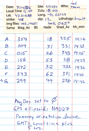
The file orient.txt is a tab delimited file which can be edited or viewed with Excel as well. Find out what the location name is for this project on the first line of the orient.txt file. [This project has only one location name.] For complete details of what you can put in the orient.txt file for your own studies, see the section on Field Information. In this tutorial we will use just a subset of the options. The numbers in the orient.txt file were entered from the notebook page written in the field by the sampling team:
For details on the SIO measurement format and other options for magnetometer files, see the section on magnetometer files. The zeq_redo file contains instructions for how to interpret the measurement data. The format is explained in the help pages for importing prior interpretations.
Begin importing data by opening a terminal window.
In the terminal window, type MagIC.py on the command line. When prompted, point the program to the (empty) MagIC directory within your project directory. If you forgot to create the MagIC directory, you can create it within the program.
Pull down the Import menu and select the "Orientation files" option. This option constructs a call to the orientation_magic.py program. Find the orient.txt file in your MyFiles directory and follow the instructions under importing orientation files.
These samples were oriented in the field with a "Pomeroy" orientation device that measures the horizontal direction of drill with a magnetic compass (and a sun compass) and the angle of drill measured in degrees from the vertical down direction (the hade), so the orientation convention is #1. Just click on the 'OK' button to keep this default value.
Because the orient.txt file has the date and location of sampling, we can have orientation_magic.py can calculate the declination correction for us, using the IGRF. So, just click on the "OK" button to keep this default option.
If you looked in the example orient.txt file itself, you might have noticed the sample name format: ns035a. The site is ns035, the sample is 'a'. So, the naming convention is #1. Just click on the 'OK' button.
In the field notebook pages above, you will find that these samples were taken during the summer in Minnesota. The time difference between local time and universal time was five hours - with universal time being ahead of local time. Therefore, enter a '-5' in the field for "Hours to subtract from local time for GMT".
The structural orientation for this study was taking from field maps published elsewhere, so the bedding dip directions were already corrected for magnetic declination. Therefore, select 'Don't correct bedding dip...' when asked.
Now we can choose some helpful method codes to describe the sampling conditions. The samples were drilled in the field, so check the FS-FD box. Samples were located using a GPS, so check the FS-LOC-GPS field and were oriented with a Pomeroy orientation device.
If you have age information for specific sites, you will want to import these now so that those ages can be attached to the sites that were dated when you prepare your data for uploading. You can do that now by selecting the "import er_ages.txt" option under the Import window. Just select the file named er_ages.txt from your MyFiles directory when prompted.
Now we start importing the measurement data. Pull down the Import menu expand the Magnetometer files menu and select "SIO format".
When prompted, choose the ns_a.mag file in your MyFiles directory. Check the AF box in the lab protocol window. Enter the location name that you found at the top of the orient.txt file (North Shore Volcanics) in the box for location name. If you looked in the file ns_a.mag you will have noticed that the specimen name is distinguished from the sample name by a terminal number. So enter a '1' on the line labeled '# characters for specimen....' and click on the 'OK' button. The naming convention for these files is the same as for the orientation files, so just click on the 'OK' button to keep the default naming convention #1.
Now import the SIO formatted file ns_t.mag. This file contains the thermal demagnetization data for the study, so check the 'T' box when prompted. Follow the same steps as for the ns_a.mag file above.
You are done importing measurement files for this study. The next step is to "Assemble measurements" under the Import menu.
Now we turn to the Data reduction menu. Select the option "Import prior interpretations" and choose the zeq_redo file in your MyFiles directory. This brings some previous interpretations into the MagIC directory and calculates the best fit directions and great circles according to the instructions in the zeq_redo file from the data in the measurement file.
Now select the Demagnetization data to inspect the previous interpretations and modify them if desired. If in practice there are no prior interpretations, you can just interpret the data. The first set of plots will look something like this:
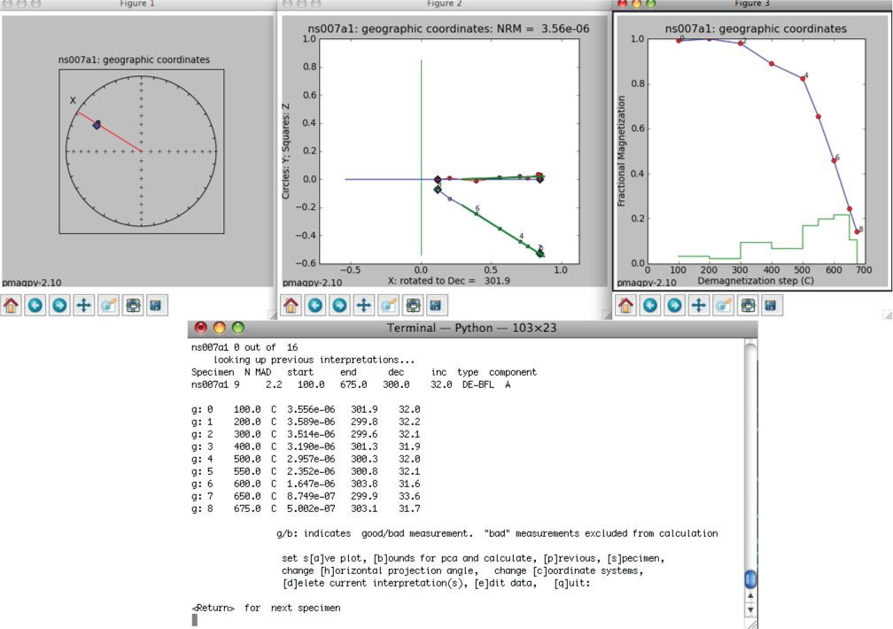
For details on how to navigate through the demagnetization diagram program (zeq_magic.py) see the Demagnetization data help link. To proceed to the next sample, click on the terminal window and hit the "Enter" (or "return") key.
When the program finishes, or you quit the program, you can re-calculate directions in all available coordinate systems (there are three in this example: specimen, geographic and tilt corrected) with the Assemble specimens command. Do this now.
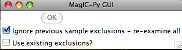
Now we can look at possible reasons for outliers in the directions by selecting "Check sample orientations" option in the Import menu. There are no previous sample exclusions, so just click on the "Ignore previous sample exclusions" button:
The check orientation option calls the program site_edit.py and steps through the data site by site, printing out sample/specimen information in the terminal window and plotting them, along with the Fisher mean and alpha_95 in the picture window. If a particular directions looks out of place, e.g., ns007b1 in the example data set shown here,
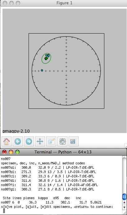
you can examine common sources of outlier directions by typing "e" in the command line window and entering the suspicious specimen name when asked. You will get a picture like this:
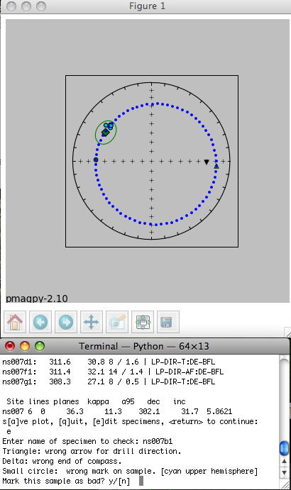
The blue dotted line traces the directions that would be generated if a stray mark on the sample was used instead of the actual drill direction - an interpretation which seems reasonable because the blue dotted line goes right through the directions from all the other specimens at the site. Therefore, type in a 'y' on the command line. And choose "bad mark" as the explanation for rejecting this sample's data. This will mark the sample_flag in the er_samples.txt file as "b" and write in the reason under the sample_description field. Stepping through all the sites allows you to throw out clearly mis-oriented data from your interpretations while preserving the data and the rationale in the database. When the program site_edit.py has finished. You will be asked to run "Assemble Specimens" which is a necessary step before you "Assemble Results". So be sure to choose "Assemble Specimens" from the Import menu before proceeding.
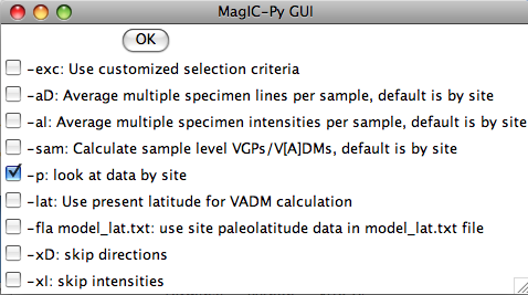
Now choose the Assemble results option. You will be asked for age bounds for this study. These rocks were part of the Keeweenawan lava flows exposed along the north shore of Lake Superior in Minnesota and are approximately 1.1 Ga, so enter 1.1 for minimum and maximum age and "Ga" in the age units line. When asked, accept the default specimen file for processing by clicking on the "OK" button. Note that for a "real" data set, you might have site level age information. This were entered into a file called er_ages.txt and imported to your MagIC project directory using the import er_ages option in the import menu. You have not (yet) customized your selection criteria, so you should not select the -exc option. Just click on the '-p' option when presented with a page that looks like this:
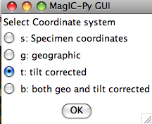
Press the radio button next to 't: tilt corrected' when asked, then click on the 'OK' button. You will be able to look at the data by site because you chose the -p option and you should get a pair of windows that look something like this:
The specimen_results_magic.py program called by this option first averages specimen data by sample (if desired), then sample (or specimen) data by site. It will print out what it is doing in the terminal window. After it finished the first site, you should see the summary site mean statistics, then details for each specimen that was used in the calculation and a plot of the data:
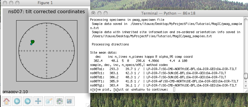
The magic_method_codes summarize how each specimen was treated. The "LP-DIR" method code tells you what type of demagnetization experiment was done (T for thermal, AF for alternating field), the "SO" code tells you about sample orientaion (sun or magnetic compass, for example), the "DE" code documents how the direction estimation was done (BFL for best-fit line or BFP for best-fit plane, for example), the "DA" code lists data adjustments (DIR-GEO, means the data were transformed to geographic coordinates and DIR-TILT means they were also adjusted for tilt). If there is a problem with a site, you can quit the program and return to demagnetization data, or any previous step to track down and fix any problems. If you are satisfied, just step through the sites (there is only one for this tutorial) and the program will finish.
If you want to change the default selection criteria - just click on the Customize Criteria option. This will allow you to tighten or loosen specimen, sample, and site level statistics for selecting data for inclusion in your final results. After you do this, you will need to re-run the Assemble specimens and Assemble results procedures explained above.
You can make various summary plots of the data using options in the Utilities menu. You can also export your results to tables suitable for including in a publication (site summary statistics, ages, site locations, etc.) by choosing the "Extract Results to Table" option under the Data Reduction menu. When you are ready to proceed to the MagIC Console software, choose the "Prepare upload text file" under the Data Reduction menu. After the program has finished, start your Excel program and open the MagIC Console software. Make a new smartbook for this project. Select the "import data" option and choose the file "upload_dos.txt" in your project MagIC directory. The data will load into the correct tables. Then, for a "real" data set, you would fill out the location, and citation tables before choosing "Prepare for upload" and uploading the data into the MagIC database.
You are now ready to try to upload your own data!
4.4.2 Rock Magnetic Study
Under construction