MagIC Help Library |
|||
|
|
|||
4 Importing Data With PmagPy and MagIC.py
The MagIC Console software allows entry of data directly into an Excel Smartbook. However, the work flow for a typical paleomagnetic study involves taking samples in the field, analyzing specimens in the laboratory and interpreting those measurements in a variety of ways. Individual laboratories use a variety of custom software packages to create plots and tables that are suitable for publication from the measurement and field data. Measurements are made on specimens which are part of samples which are part of sites and this context must be preserved explictly in the MagIC database tables. Also, measurements can be done on a variety of instruments, under different conditions of pre-treatment, measuring temperatures, frequencies, orientations, etc. These details must also be preserved in the database for the measurement data to have any value. To facilitate the process of analyzing and importing paleo- and rock magnetic data and meta-data into the MagIC console, we have written the PmagPy software package.
PmagPy is written in the Python Programming Language. Python is flexible, freely available, cross platform, widely used and well documented and much easier to read and learn than Perl. It has many numerical or statistical tools 3D visualization is improving all the time. And it is free. As of this writing, PmagPy comprises 135 programs which perform a variety of tasks from simple calculations to creating complicated plots. These call on functions in several modules: the plotting module, pmagplotlib does the heavy lifting for creating plots and pmag has most of the functions performing calculations. Details on how to use the complete software package and the source code are available through the PmagPy home page.
PmagPy programs are called from the command line and uses switches to set key parameters. Most paleomagnetists are not Unix oriented and dislike the command line interface. For this reason, we have written a graphical user interface (GUI) called MagIC.py. MagIC.py allows importing of field and measurement data for a variety of laboratory conventions into the MagIC format. It also allows plotting and interpretation of the data and preparation of all the data files into to text file that can be directly imported into the MagIC console.
4.1 Installation of PmagPy
Python can be painful to install (but so can all other programming environments). The Enthought Python Distribution is a comprehensive version that contains all of the packages used by PmagPy. It is also relatively straight-forward to install. Follow the instructions for your platform (exactly!) described on the PmagPy website. Then install the PmagPy package as instructed. Be sure to set your path correctly. If high resolution maps are desired, you can also install the high resolution database for the basemap module.
4.1.1 Finding a command line prompt in a terminal window
If you are not using a UniX like computer, you may never have encountered a command line. While the MagIC.py Graphical User Interface (GUI) is an attempt to make life as easy for you by constructing UNIX commands for you, you still need to find the command line to start it up.
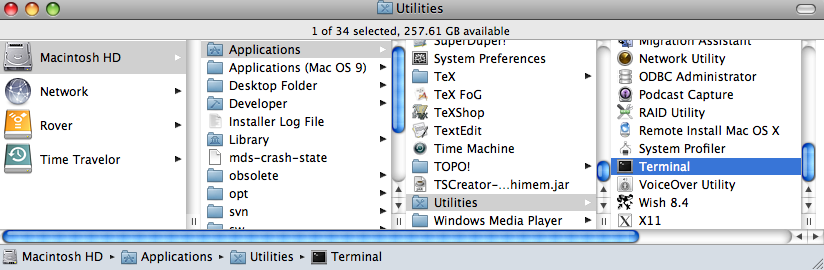
Under the MacOS X operating system, you may have two choices: Terminal and X11. These reside in the Utilities folder within the Applications folder:
Under the Windows operating system, find the program called: Command Prompt in the Start menu:
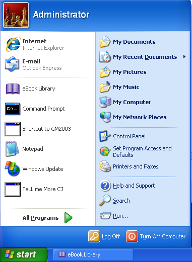
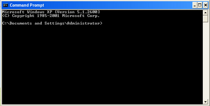
Note that the location of this program varies on various computers, so you may have to hunt around a little to find yours. Also, the actual "prompt" will vary for different machines. A windows prompt window looks something like this:
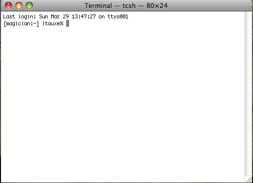
Under Unix operating systems (including MacOS), the prompt is a "%" (c-shell) or a "$" (bash). We will use a "%" to indicate the prompt in these help pages. This is a picture of the command window using the c-shell. The prompt has been customized to show the machine name (magician) and the user name (ltauxe).
In these help pages, we will refer to the command line on which you type and the terminal window in which it is located.
4.1.2 Testing installation
To test if the installation was successful, find your command line prompt in a terminal window. Type in the window:
fishrot.py -I 45 >delete.me; eqarea.py -f delete.me
followed by a carriage return or enter key. You should have something that looks similar to this (details will vary!):
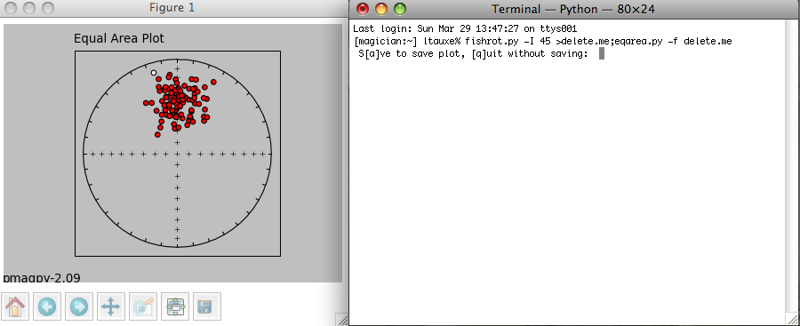
The command fishrot.py creates a fisher distribution with a mean inclination of 45o and saves it in a file called delete.me. eqarea.py makes a plot of it. The tag pmagpy-2.09 in the lower left hand corner is the PmagPy version number that created the plot. You can save the plot in a variety of formats by clicking on the disk icon on the tool bar of the picture (right hand one). Specifying the format name by using the desired suffix in the file name. For example, a file name of myplot.svg would save as an svg format, myplot.png in a png format, etc. The default file format is .svg. Complete details of these and other programs are available through the PmagPy home page.
4.2 Getting Ready for MagIC.py
4.2.1 Setting up a Project Directory
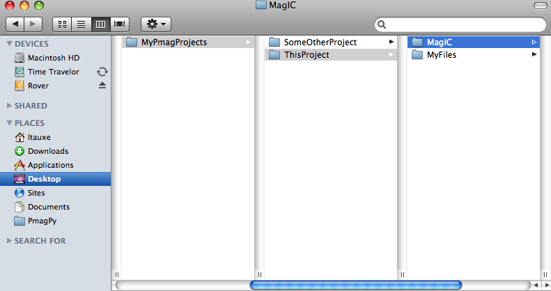
PmagPy uses a number of default file names. While these can be customized by the expert user, it is preferable to keep the MagIC files for a each paleomagnetic study in separate directories. For each study, create a directory with a name that relates to that study. Here we will call it ThisProject. This directory should have NO SPACES in the name and be placed on the hard drive in a place that has NO spaces in the path. Under Windows, this means you should not use your home directory, but create a directory called for example: D:\MyPmagProjects and place ThisProject in that directory.
Inside ThisProject, create two additional directories: MyFiles and MagIC. All the files that you want to import into the MagIC format should be placed in MyFiles and you should just leave MagIC alone unless you really know what you are doing.
Your Directory tree might look like this now:
4.2.2 Field Information
Paleomagnetists collect samples in the field and record orientation, location and lithology, etc. in field notebooks. This information is necessary for placing the data into a well characterized context and should be included in the MagIC contribution. Importing field data into the MagIC format using PmagPy requires you to fill in a tab delimited text file with a particular format, here called the "orient.txt" format. These should be placed in the MyFiles directory in the Project directory. When importing the data, you must figure out how your orientation and name schemes relate to what MagIC expects. The process is difficult because there are a multitude of possible naming conventions which relate specimen to sample to site, orientation conventions which convert specimen measurements in geographic and stratigraphic coordinates, etc. PmagPy supports a number of conventions and more can be added by Request. Here we go through each of these problems, starting with the orient.txt file format, and then covering sample orientation and naming schemes.
First of all, separate your sampling information into the locations that you plan to designate in the data base. Location name (er_location_name) in MagIC is a rather loosely defined concept which groups together collections of related sites. A location could be for example a region or a stratigraphic section. Location names are useful for retrieving data out of the MagIC database, so choose your location names wisely. Each orient.txt format file contains information for a single location, so fill one out for each of your "locations".
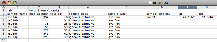
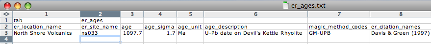
The First Line of the orient.txt file contains two tab delimited fields. The first is the word 'tab' and the second is the location name, in this example it is North Shore Volcanics. Use the same location name EVERY TIME you are asked for it for data related to this collection of samples.
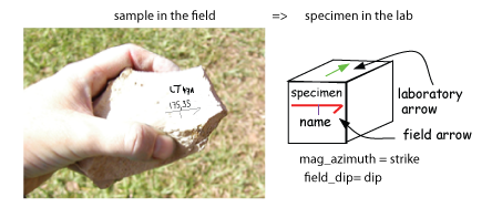
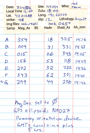
The Second Line of the orient.txt file has the column names. The order of the columns doesn't matter, but the names of the columns do. Some of these are required and others are optional. The example above shows all the REQUIRED fields. Note that latitude and longitude are specified in decimal degrees. mag_azimuth and field_dip are the notebook entries of the sample orientation. Sample class, Lithology and Type are Controlled MagIC Vocabularies, so enter colon delimited lists as appropriate. Also, notice how some fields are only entered once. The PmagPy program (orientation_magic.py) assumes that the last encountered value pertains to all subsequent blank entries.
Optional Fields in orient.txt formatted files are: [date, shadow_angle, hhmm], date, stratigraphic_height, [bedding_dip_direction, bedding_dip], [image_name, image_look, image_photographer], participants, method_codes, site_name, and site_description, GPS_Az
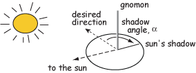
For Sun Compass measurements, supply the shadow_angle, date and time. The date must be in mm/dd/yy format. Be sure you know the offset to Universal Time as you will have to supply that later. Also, only put data from one time zone in a single file. The shadow angle should follow the convention shown in the figure:
All images, for example outcrop photos are supplied as a separate zip file. image_name is the name of the picture you will import, image_look is the "look direction" and image_photographer is the person who took the picture. This information will be put in a file named er_images.txt and will ultimately be read into the er_image table in the console where addiional information must be entered (keywords, etc.).
Often, paleomagnetists note when a sample orientation is suspect in the field. To indicate that a particular sample may have an uncertainty in its orientation that is greater than about 5o, enter SO-GT5 in the method_codes column and any other special codes pertaining to a particular sample from the method codes table. Other general method codes can be entered later. Note that unlike date and sample_class, the method codes entered in orient.txt pertain only to the sample on the same line.
If there is not a supported relationship between the sample_name and the site_name (see sample naming schemes below), you can enter the site name under site_name for each sample. For example, you could group samples together that should ultimately be averaged together (multiple "sites" that sampled the same field could be grouped under a single "site name" here.
Supported sample orientation schemes:
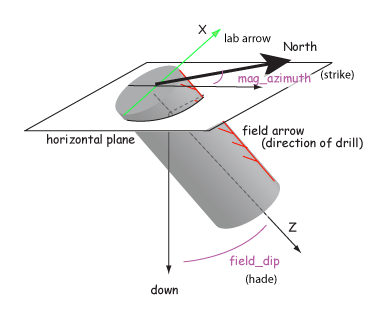
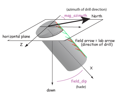
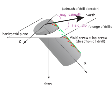
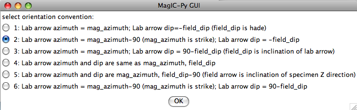
Samples are oriented in the field with a "field arrow" and measured in the laboratory with a "lab arrow". The lab arrow is the positive X direction of the right handed coordinate system of the specimen measurements. The lab and field arrows may not be the same. In the MagIC database, we require the orientation (azimuth and plunge) of the X direction of the measurements (lab arrow). Here are some popular conventions that convert the field arrow azimuth (mag_azimuth in the orient.txt file) and dip (field_dip in orient.txt) to the azimuth and plunge of the laboratory arrow (sample_azimuth and sample_dip in er_samples.txt). The two angles, mag_azimuth and field_dip are explained below.
[1] Standard Pomeroy convention of azimuth and hade (degrees from vertical down) of the drill direction (field arrow). sample_azimuth = mag_azimuth; sample_dip =-field_dip.
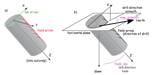
[2] Field arrow is the strike of the plane orthogonal to the drill direction, Field dip is the hade of the drill direction. Lab arrow azimuth = mag_azimuth-90o; Lab arrow dip = -field_dip
[3] Lab arrow is the same as the drill direction; hade was measured in the field. Lab arrow azimuth = mag_azimuth; Lab arrow dip = 90o-field_dip.
[4] Lab arrow orientation same as mag_azimuth and field_dip.
[5] Same as AZDIP convention explained below - azimuth and inclination of the drill direction are mag_azimuth and field_dip; lab arrow is as in [1] above. field arrow are lab arrow azimuth is same as mag_azimuth, Lab arrow dip = field_dip-90o
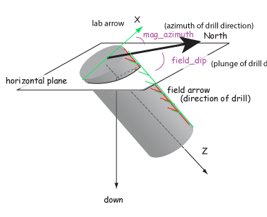
[6] Lab arrow azimuth = mag_azimuth-90o, Lab arrow dip = 90o-field_dip, i.e., field arrow was strike and dip of orthogonal face:
Supported sample naming conventions:
Structural corrections:
Because of the ambiguity of strike and dip, the MagIC database uses the dip direction and dip where dip is positive from 0 => 180. Dips > 90 are overturned beds. Plunging folds and multiple rotations are handled with the pmag_rotations table and are not implemented within PmagPy.
4.2.3 Measurement Data
The MagIC database is designed to accept data from a wide variety of paleomagnetic and rock magnetic experiments. Because of this the magic_measurements table is very complicated. Each measurement only makes sense in the context of what happened to the specimen before measurement and under what conditions the measurement was made (temperature, frequency, applied field, specimen orientation, etc). Also, there are many different kinds of instruments in common use, including rock magnetometers, susceptibility meters, Curie balances, vibrating sample and alternating gradient force magnetometers, and so on. We have made an effort to write translation programs for the most popular instrument and file formats and continue to add new supported formats as the opportunity arises. Here we describe the various supported data types and tell you how to prepare your files for importing. In general, all files for importing should be placed in the MyFiles directory or in subdirectories therein as needed.
Rock magnetometer file formats
Rock Magnetometer File Formats:
Supported files and how to prepare for importing:
CIT format: The CIT format is the standard format used in the paleomagnetics laboratory at CalTech and other related labs. This is the default file format used by the PaleoMag software package. This data format stores demagnetization data for individual specimens in separate sample data files. The format for these is described on the PaleoMag website. The file names with specimen data from a given site are listed in a .SAM file along with other information such as the latitude, longitude, magnetic decliantion, bedding orientation, etc. Details for the format for the .SAM files are located here. Place all the files (sample data files and summary .SAM files) in your MyFiles directory and proceed to the section on MagIC.py.
HUJI format:
The HUJI format is the standard format used in the paleomagnetics laboratory at Hebrew University in Jerusalem.
Under contstruction
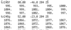
LDEO format:
The LDEO format is the standard format used in the paleomagnetics laboratory at Lamont Doherty Earth Observatory and other related labs. Here is an example:
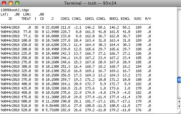
The first line is the file name. The second has the latitude and longitude for the site. The third is a header file with column labels. These are: the specimen name, a treatment key, and instrument code, intensity in 10-4 emu, CDECL and CINCL which the declination and inclination in specimen (core) coordinates. Optionally, there are GDECL, GINCL which are declination and inclination in geographic coordinates, BDECL, BINCL which are in stratigraphic coordinates, SUSC which is susceptibility (in 10-6 SI). Data in this format must be separated by experiment type (alternating field demagnetization, thermal demagnetiztation). Place all data files in your MyFiles directorty and proceed to the section on MagIC.py.
LIV-MW format:
The LIV-MW format is the format used for microwave data in the paleomagnetics laboratory at Liverpool.
Under contstruction
SIO format: The SIO format has six required columns: Specimen_name Treatment_code Uncertainty Intensity Declination Inclination. These are in a space delimited file with no header.
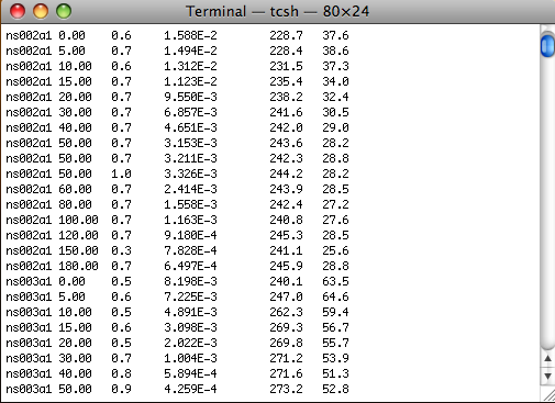
The specimen name is assumed to have a simple relationship to the sample name using characters at the end of the specimen name. All data in a given file must have the same number of characters relating specimen to sample. For example, in the specimen name ns002a1, the terminal number is the specimen number of sample ns002a. If there are many specimens (more than 10, say), one might have a specimen ns002a01, in which case the last two characters are the specimen identifier. All data in a given file must have the same number of characters that serve as the specimen ID. The relationship of the sample name to site name can follow the sample naming convention described in the section on Field Information.
The treatment code specifies the treatment step as well as information about applied fields or even sometimes orientation during treatment (e.g., during an AARM experiment). The treatment code has the form XXX.YYY where YYY is a variable length modifier that can range from zero to three characters in length. For simple demagnetization experiments, the treatment is either the temperature (in Centigrade) to which the specimen was heated and cooled in zero field prior to measurement or the alternating field (in millitesla) to which the specimen was subjected in zero field prior to measurement.
Measurement uncertainty is the circular standard deviation of repeated measurements at the same treatment step (usually in different orientations in the magnetometer.)
Intensity is assumed to be total moment in emu (kAm2).
Declination and inclination are in specimen coordinates.
The optional meta-data string is of the form:
mm/dd/yy;hh:mm;[dC,mT];xx.xx;UNITS;USER;INST;NMEAS
where: hh is in 24 hour, dC or mT units of treatment XXX (see Treatment code above) for thermal or AF respectively, xx.xxx is the DC field, UNITS is the units of the DC field (microT, mT), INST is the nstrument code, number of axes, number of positions (e.g., G34 is 2G, three axes, measured in four positions), and NMEAS is the number of measurements in a single position (1,3,200...).
Treatment codes for special experiments:
XXX.0 first zero field step
XXX.1 first in field step [XXX.0 and XXX.1 can be done in any order]
XXX.2 second in-field step at lower temperature (pTRM check)
XXX.3 second zero-field step after infield (pTRM check step)
XXX.3 MUST be done in this order [XXX.0, (optional XXX.2), XXX.1 XXX.3]
X.00 baseline step (AF in zero bias field - high peak field)
X.1 ARM step (in field step) where X is the step number in the 15 position scheme described here.
XXX.YYY XXX is temperature step of total TRM and YYY is dc field in microtesla.
UB format:
The UB format is the standard format in the University of Barcelona Laboratory and is the 2G binary format. These cannot be viewed with a text editor.
Under construction
UU format:
The UU format is the standard format in the University of Utrecht Fort Hoofddijk Laboratory that is used by the PalMag software package.
Under construction
UCSC format:
Two University of California Santa Cruz formats are supported - the new standard and a legacy file format.
Under construction
2G format: 2G Enterprises ships magnetometers with software that saves data in a binary "2G" format. Each file has the data for a given specimen and must have ".dat" or ".DAT" as a file type (e.g., Id1aa.dat).
PMD (ascii) format:There are two formats called '.PMD': an ascii file format used with the software package of Randy Enkin and a binary format. Both are used with the PaleoMac program written by J.P. Cogne. The ASCII file format is the so-called I.P.G. format described on the PaleoMaC web site. The two different file formats, so be sure you know which one you are using. Here is an example of the ascii (I.P.G., AF) file format:
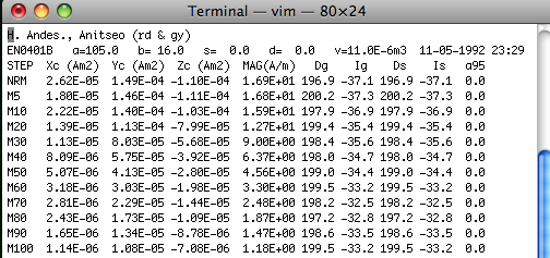
The first line is a comment and the second line has: SPECIMEN a=AZIMUTH b=HADE s= STRIKE d= DIP v=VOLUME DATE TIME. The orientation information AZIMUTH and HADE are of the specimen's 'X' direction (orientation convention #1 in our convention). The third line is a header. The remaining lines are the measurement data. The first column specifies the treatment step: NRM, MXX or TXX. M steps are AF demagnetizing peak fields in mT and T steps are thermal demagnetization temperatures in oC. Columns 2-4 are the X,Y,Z data in specimen coordinates. These are in Am2. Column 5 is the volume normalized magnetization in A/m. Columns 6 and 7 are the Declination and Inclination in geographic coordinates and Columns 8 and 9 are the same in tilt corrected (stratigraphic) coordinates. There are optional columns for alpha95 and susceptibility.
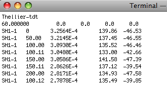
ThellierTool (tdt) format: Here is an example of a TDT formatted file:
To use this option, place all .tdt files in a directory. You will be asked the usual questions about location, and naming conventions. MagIC.py copies each input file into the MagIC Project directory and generates a command to the program TDT_magic.py which creates a magic_measurements formatted file with the same name, but with a .magic extension. It writes and entry to the measurements.log file so that all the .magic files can be combined when you assemble your measurements. Note that all files in a given directory must have the same location and naming conventions.
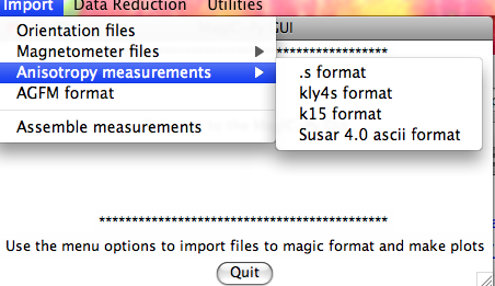
Anisotropy of Magnetic Susceptibility File Formats:
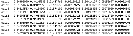
.s format: The ".s" option allows strings of data with the format: X11 X22 X33 X12 X23 X13 where the Xii are the tensor elements (remembering that X12=X21, X23=X32 and X13=X31):

There is an optional first column with the specimen name and an optional last column with the standard deviation of the measurements (calculated with the Hext method). Here is an example of a file with the optional specimen name and standard deviation columns:
For more on how to measure AMS and calculate tensor elements, see the online textbook chapters of Essentials of Paleomagnetism.
Kly4S format: This data file format is generated by the program described by Gee, J.S., Tauxe, L., Constable, C., AMSSpin: A LabVIEW program for measuring the anisotropy of magnetic susceptibility with the Kappabridge KLY-4S, Geochem. Geophys. Geosyst., 9, Q08Y02, http://dx.doi.org/10.1029/2008GC001976, 2008. It is essentially the same as the .s format (with specimen name in the first column), but has much more information about the frequency, appied field, date and time of measurement, and so on:
k15 format: The .k15 format has the following format:
The first row for each specimen contains the specimen name, the azimuth and plunge of the measurement arrow and the strike and dip of the rock unit. The following three lines are the 15 measurement measurement scheme used with the Kappabridge instruments in static mode.
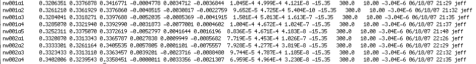
Susar 4.0 ascii format:
This format is generated by the Susar 4.0 program used for running Kappabridge instruments in spinning mode. It is the default program that comes with the instrument. Here is an example of an output file:
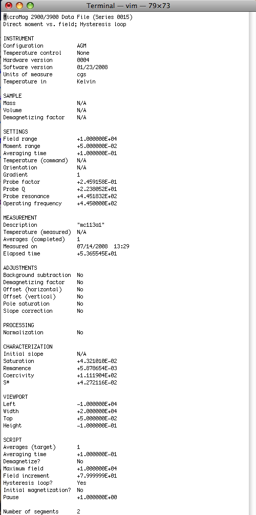
Hysteresis file formats:Hysteresis data can be obtained on a wide variety of instruments from vibrating sample magnetometers (VSM), alternating gradient force magnetic force magnetometers (AGFM), MPMS instruments, etc. As of now, only AGFM data from Micromag instruments are supported and only two of the many possible experiments are supported (basic hysteresis loop and "back-field" curve). These experiments have two different styles of header, the orignal and the "new". Here are some examples:
Basic hysteresis loop:This is an example of the original file format for a "basic" loop".
Back-field curve:This is an example of the original file format for a back-field curve.
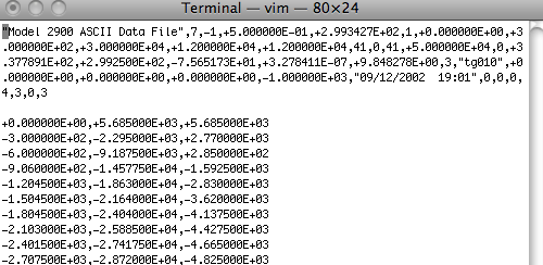
New: Both of these experiments can also be saved with the "new" format. Here is an example of the "new" header:
4.3 Using the MagIC.py GUI
The MagIC.py graphical user interface is a Python program that facilitates importing of measurement data and sample information (location, orientation, etc.) into the MagIC format and interpretation thereof. It will help prepare all the files into a text format that can be imported directly into a MagIC smartbook. MagIC.py copies files to be uploaded into a special project MagIC directory, translates them into the MagIC format and keeps track of things in various log files. For this reason, once the project MagIC directory has been created, you should just leave it alone. See the help pages for instructions on setting up the Project directories and installing PmagPy if you have not yet done so. Once you have placed all the needed files (orient.txt formatted files for each location and the measurement data files) in the MyFiles directory, open up a terminal window and type MagIC.py on the command line. Select the MagIC directory in your Project directory when prompted.
If at any time it seems that the MagIC.py GUI is unresponsive or "stuck", click on the Python icon and try again. I think this only happens on Macs, so look on your Dock for the python symbol:

4.3.1 File Menu
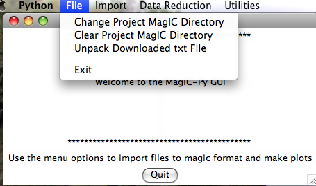
Different operating systems will have a different look, but all versions will put up a Welcome window when you have fired up the program MagIC.py. When you pull down the "File" menu, you will see these options:
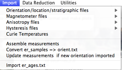
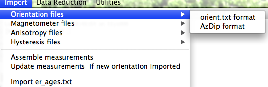
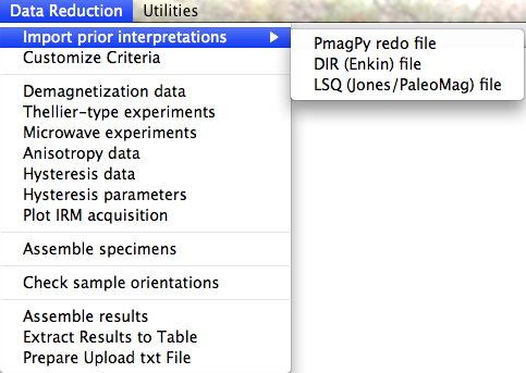
4.3.2 Import Menu
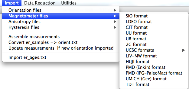
When you pull down the "Import" menu, you will see these options:
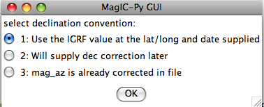
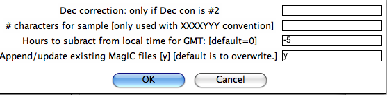
If none fit, then do the transformation yourself and provide the azimuth and plunge of the "X" axes used in your measurements and choose convention #4. Click on the "OK" button to advance to the next window. This will ask you about your preferences for correcting for magnetic declination. The declination used to correct your magnetic compass data will be recorded in the sample_declination_correction field of the er_samples table. If you set your magnetic declination correction to zero in the field and provided the date, latitude and longitude of the sampling location, you can request that orientation_magic.py calculate the declination correction from the (D)IGRF value. It uses the IGRF-10 coefficients which can be downloaded from the National geophysical data center website. Alternatively, you can supply your preferred value on a later page (option 2), or supply magnetic azimuth data that have already been corrected (option 3):
On the next page, you must select your naming convention. Note that for options #4 and 7, the number of characters that distinguish sample from site will be supplied on a later page. If none of these options fit your naming convention, put the site name under the column heading site_name in the orient.txt file. This can also be used to group samples that you wish to average together as a "super-site" mean, assuming that they record the same field state (averaging sets of sequential lava flows, for example.)
Often a the attitude of the rock units sampled for paleomagnetic study will be oriented multiple times. To average these, one would convert the bedding directions to bedding poles, take a fisher mean of the poles, then convert the mean bedding pole back to dip direction and dip. If you want to do that with the bedding information in the file you are importing, check the box "Take fisher mean of the bedding poles" in this window:
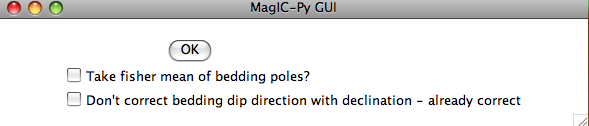
Check the box marked 'Don't correct bedding dip direction with declination....' if you corrected the bedding dip directions for declination already. (It is possible that the bedding dip directions be corrected while the sample orientations are not, for example if the bedding attitudes were read off an existing map...).
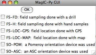
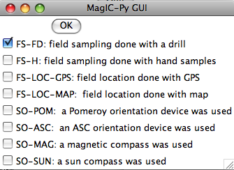
The next window allows you to select method codes that describe sample conditions. Select all that apply to all samples. Sample specific method codes can be attached within the orient.txt file itself.
After you get through all the windows, the MagIC.py GUI will generate commands which will appear on your command line prompt. It copies the orient.txt formatted file into the MagIC directory and calls the program orientation_magic.py. This program reads your datafile and parses the information into several MagIC tables (usually er_samples.txt, er_sites.txt, but also er_images.txt if you entered image information in the orient.txt file). If you indicated that you had multiple locations, it will append each subsequent import file to these same filenames. Check the terminal window for errors! If you can't figure out what went wrong, send a screen shot and the offending orient.txt file and I'll try to figure out what went wrong.
SIO formatted files: In the first window, choose the laboratory protocol from the following menu:
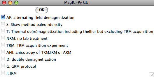
Check all that apply: AF indicates that the data are from an alternating field demagnetization experiment. If a double or tiriple (GRM) demagnetization protocol was followed, also check the D and G boxes. For thermal demagnetization and also double heating paleointensity experiments, check the 'T' box. Do not check this box, however, if the data are from a TRM aquisition experiment (multiple field steps with total TRMs). If these data are some form of anisotropy experiment, check the ANI box and if they are IRM data, check the IRM box.
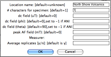
Enter a variety of important information in the next window:
Now you must choose your naming convention. NB: All specimens must have the same naming convention within a single file. After collecting all the required information, MagIC.py generates a call to the program mag_magic.py which sorts the measurement data out into the MagIC format. Each imported file is stored as a file of the same name as the input file, but with .magic appended to the end. Check the terminal window for errors. It will also let you know about all the averaging that has taken place - these comments are not errors. After all the measurement files have been imported, select "Assemble measurements" from the Import pull down window. You are now ready for "Data reduction".
Other formats:
LDEO format:
CIT format:
UU format:
UB format:
2G format: To use this option, first place all the 2G binary .dat files in a separate sub-directory within your MyFiles directory. All the files in a given sub-directory must have the naming convention, sampling meta-data and location name. You will first be asked to specify the directory to import and then the naming convention (see instructions for .PMD files below). Be sure to assemble your measurements before attempting to make plots from them.
UCSC format:
LIV-MW format:
HUJI format:
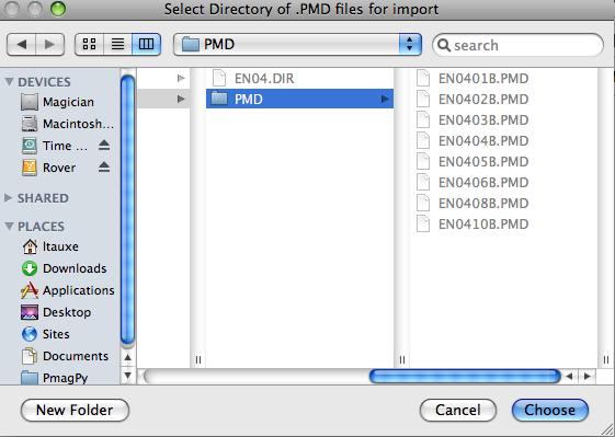
PMD (ascii) format: To use this option, first place all the .PMD formatted file in a separate sub-directory within your MyFiles directory. All the files in a given directory must have the same naming convention, sampling meta-data and location name. You will first be asked to specify the directory to import:
Then you will be asked to specify the naming convention that you have used. Additional information can be supplied in the table:
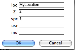
Notice that because if you specified naming conventions #4 or #7. (e.g., specimen EN0401B is from sample EN0401 and from site EN04), we must supply the number of characters designating sample from site here (2), as well as the number of characters designating specimen from sample (1). We can specify some of the sampling conventions using the magic method codes on this page:
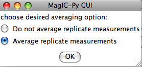
Normally, you should elect to average replicate measurements at a given treatment step, but some studies you may not want to, so you are given the option here:
If you have already imported orientation information and created a file called er_samples.txt, the program will ask you if you want to append this information to that file (updating any existing sample orientation information in the process) or to create a new file, overwriting all existing information. This option allows you to keep .PMD files from separate locations in different directories, uploading them separately and combining all the information together into your er_samples.txt and magic_measurements.txt files. When you are finished uploading measurement data, select the Assemble Measurements option so that you can plot the data.
PMD (IPG-PaleoMac) format: You will first be asked to specify the import file, then you will be asked to specify the naming convention that you have used. Additional information can be supplied in the table:
Normally, you should elect to average replicate measurements at a given treatment step, but some studies you may not want to, so you are given the option here:
If you have already imported orientation information and created a file called er_samples.txt, the program will ask you if you want to append this information to that file (updating any existing sample orientation information in the process) or to create a new file, overwriting all existing information. This option allows you to keep files from separate locations in different directories, uploading them separately and combining all the information together into your er_samples.txt and magic_measurements.txt files. When you are finished uploading measurement data, select the Assemble Measurements option so that you can plot the data.
TDT (ThellierTool) format: This option allows input of the ThellierTool format for double heating experiments. You will be asked all the usual questions regarding the directory in which the .tdt files reside, the naming convention, and the location name. Be sure that each directory contains files with the same location and naming conventions. MagIC.py will copy each file into the MagIC Project directory and generate a command to the program TDT_magic.py which does the conversion to a magic formatted measurement file. When you are finished, select "Assembls Measurements" and proceed to viewing of Thellier data under the "Data Reduction" menu.
All options generate commands, depending on the file type, which create MagIC formatted files, in particular the rmag_anisotropy.txt format file which is used by the plotting programs for AMS (see Data reduction).
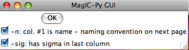
.s format: This option imports .s formatted files. After choosing the file for import, the GUI will allow you to specify if you have the specimen name in the first column and a sigma value in the last:
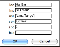
KLY4s format: This option imports KLY4s formatted files. These files are essentially enhanced .s files and this option has enhanced features. If you have imported orientation information it will do the transformations from specimen to geographic and stratigraphic reference frames which can then be plotted with the anisotropy plotting options. If you have not imported orientation information, the program will complain, but go ahead with the importation - note that the other reference frames will not be available until you re-import the KLY4s file. You will be asked to specify your naming convention and supplemental information:
Type in your "location" on the line labeled 'loc', the number of characters used to differentiate between specimen and sample, who made the measurements (optional) and on what instrument (optional) in the "usr" and "ins" lines. The GUI first copies your data file into the MagIC project directory and then constructs a call to kly4s_magic.py on the command line. Check the terminal window for errors! Be sure to "assemble measurements" before attempting to plot your data.
K15 format: This option imports K15 formatted files. These files have the orientation information embedded in them. If you have not already imported orientation information for a particular sample, the embedded information will be added to the existing er_samples.txt file. If none exists, a new er_samples.txt file will be created. You will be asked to specify your naming convention and usual supplemental information. Type in your "location" on the line labeled 'loc', the number of characters used to differentiate between specimen and sample, who made the measurements (optional) and on what instrument (optional) in the "usr" and "ins" lines. The GUI first copies your data file into the MagIC project directory and then constructs a call to k15_magic.py on the command line. Check the terminal window for errors! Be sure to "assemble measurements" before attempting to plot your data.
SUSAR ascii format: This option imports SUSAR ascii formatted files. These files have the orientation information embedded in them. If you have not already imported orientation information for a particular sample, the embedded information will be added to the existing er_samples.txt file. If none exists, a new er_samples.txt file will be created. You will be asked to specify your naming convention and usual supplemental information. Type in your "location" on the line labeled 'loc', the number of characters used to differentiate between specimen and sample, who made the measurements (optional) and on what instrument (optional) in the "usr" and "ins" lines. The GUI first copies your data file into the MagIC project directory and then constructs a call to k15_magic.py on the command line. Check the terminal window for errors! Be sure to "assemble measurements" before attempting to plot your data.
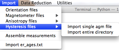
When you expand the "Hysteresis files" menu, you are presented with several choices:
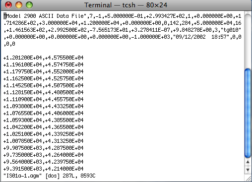
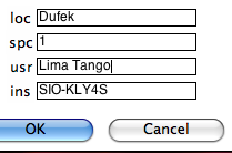
Import single agm file: This option constructs a call to the agm_magic.py program. You will first be asked to select the file for importing. This file can be in either the old or the new format - the program can figure out which automatically. Then the program requests that you select the most appropriate naming convention. These relate sample names to site and location names. The first five options are useful if there is a simple relation ship between sample and site names and all the files come from a single location. Option #6 allows you to have more complicated relationships between samples, sites and location names by specifying these "by hand" in an er_samples.txt file in your MagIC project directory. If you imported orientation information using an orient.txt file, by specifying the site name for each sample under a column labeled site_name, and importing multiple orient.txt formatted files for the individual locations involved in the study, your er_samples.txt file will already be available to you for this option. The final option is for "synthetic" specimens. Choose this if there is no "site" or "location" information and the sample is only of rock magnetic interest. Next you will be asked for additional information, for example, location name, number of characters that distinguish specimen from sample, the specimen name, etc.
Check your terminal window for specific definitions. Note that agm_magic.py assumes that the input file name had the specimen name as the root, but you can change the specimen name on the line labelled 'spn'. In this example there are two characters that distinguish the specimen (IS01a-1) from the sample (IS01a) and the naming convention was #1 (IS01a is a sample from site IS01). The program copies your data file into the MagIC project directory and calls agm_magic.py with switches set by answers to the queries set by the GUI. The actions can be viewed in your terminal window. agm_magic.py will create an output file with the same name as your input file, but with the .magic extention and write this file name to the measurements.log file. Note that if this is a "backfield" IRM experiment, you should type 'y' into the data entry window on the line labelled 'bak'.
Import entire directory: This option is very similar to the "single agm file" option described above - but allows automatic import of all files within a specified directory. The differences are that all files must have the specimen name as the file name root, and they must all have the same naming convention as you will only be asked once for all the information.
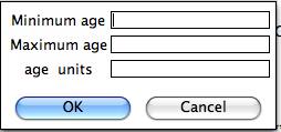
It is very important that you attach the proper method codes to your age information, so check the "Geochronology Methods" options carefully. Also, you will want to include the proper references in the er_citation_names field. You can add the citation information within the MagIC Console after your data get imported into it. To import the age file into the MagIC project directory, place the er_ages.txt file in your MyFiles directory and select the "import er_ages.txt" option in the Import menu.
4.3.3 Data Reduction Menu
When you pull down the "Data reduction" menu, you will see these options:
The zeq_redo file contains instructions for how to interpret measurement data for a standard demagnetization experiment. The first column is the specimen name, the second is the directional estimation method codes (DE-BFL for best-fit lines, DE-BFP for best-fit planes and DE-FM for Fisher means). The third column is the beginning demagnetization step for the calculation and the fourth is the end. Please note that these must be in the units required by the MagIC database, so are tesla for AF demagnetization and kelvin for thermal demagnetization. All magnetometer data are translated into these units. To convert mT to tesla, multiply by 10-3, Oe to tesla, multiply by 10-4 and from degrees C to kelvin, add 273. The fifth column is an optional component name. If none are supplied, the first interpretation for a given specimen is named "A" and the second is named "B", etc.
The thellier_redo file contains instructions for how to interpret measurement data for a double heating paleointensity experiment. The first column is the specimen name, the second is the beginning demagnetization step for the calculation and the third is the ending demagnetization step. Units must be in oC. To convert from degrees C to kelvin, add 273.
When you select the "PmagPy redo" option, the MagIC.py GUI copies the redo file into your project MagIC directory and executes the commands zeq_magic_redo.py or thellier_magic_redo.py, depending on what you imported. This program hunts through measurement data (in the magic_measurements.txt file) for data matching each specimen name, collects the data between the two end points specified in the redo file and does the desired calculation. The specimen calculations are written to a pmag_specimen formatted file called either zeq_specimens.txt or thellier_specimens.txt within your project MagIC directory. These interpretations will be read in when you try the Demagnetization data or Thellier-type experiments as described below.
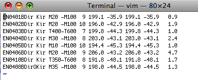
The DIR (ASCII) format is a file format used by the PaleoMac program developed at IPG by J.-P. Cogne. Here is an example of the ASCII version of these files:
The meanings of the various columns is described on the PaleoMac website. This option copies the selected file to the MagIC project directory and generates a call to the program DIR_magic.py. This translates the file into a zeq_redo formatted file (see above) called DIR_redo. It then called zeq_magic_redo.py to make a file called zeq_specimens_DIR with the MagIC formatted specimen directions in it. Note: this will overwrite any "DIR_redo" file already imported, so put ALL your interpretations into a single .DIR file! To assemble different specimen direction files together, choose "Assemble Specimens" as described below.
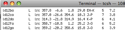
The LSQ format imports the interpretions stored in the .LSQ files output by the Craig Jones program PaleoMag and described on this website. Here is an example of the data format:
To use this option efficiently concatenate all the .LSQ files from a particular study into a single .LSQ file. You can do this by typing the command: cat *.LSQ >myLSQ on your command line if you are in the directory in which all the .LSQ files are located. Alternatively, you can import each .LSQ file individually. On choosing this option, you are asked to specify the file name to be imported and then whether or not you want to overwrite your previous specimen interpreation files. If you are importing all the interprations in a single .LSQ file (recommended), you should select the "overwrite" radio button. If you don't, you will generate a file called zeq_specimens_LSQ.txt which you can select when assembling your results.
The LSQ option first copies the .LSQ file into your MagIC project directory, then calls the program LSQ_redo.py. This program does two things: it creates a zeq_redo formatted file (see above) and it modifies the magic_measurements.txt file to mark the sample_flag to 'b' for bad for the excluded data points as indicated in the .LSQ file. Then the MagIC GUI generates pmag_specimen formatted file. You then should select "assemble specimens" and check your interpretations using the "Demagnetization Data" plotting option described below.
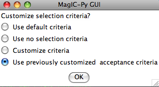
The first window allows you to specify what sort of criteria file you want to create:
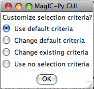
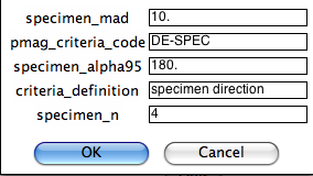
You can either use the default criteria or change them to suit your own needs. You can modify a criteria file you created before or apply no selection criteria. For changing default of existing criteria, you will then be asked to customize a series of criteria. The first is for choosing directional data for specimens:
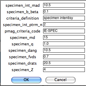
Next you can select criteria for intensity data at the specimen level:
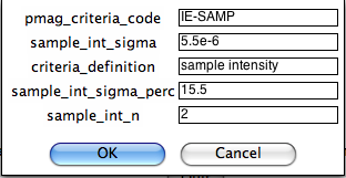
Next you can select criteria for directional data at the sample level (based on averages of multiple specimens:
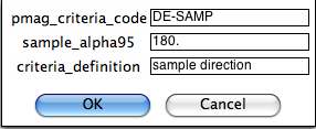
Next you can select criteria for directional data at the sample level (based on averages of multiple specimens:
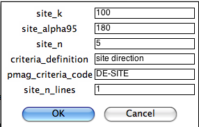
On the next page, you can customize the same parameters but for the site level:
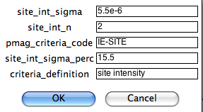
Here you customize your criteria for site level directions:
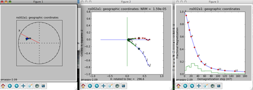
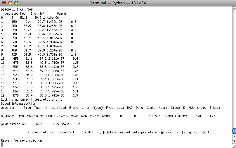
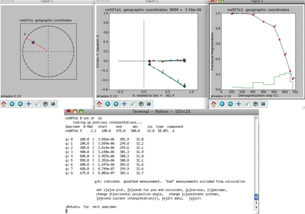
The left-hand plot is an equal area projection of the demagnetization data. The title is the specimen name and the coordinate system of the plot. Solid symbols are lower hemisphere projections. The directions of lines fit through the data are shown as blue diamonds. Green dotted lines (not shown) are the lower hemisphere projections of a best-fit plane while cyan is on the upper hemisphere. The red line is the X direction (NRM) of the middle plot.
The middle plot is a vector-end point diagram. The magnetization vectors are broken down into X,Y,Z components (depending on the coordinate system). The default for this plot is to rotate the X direction such that it is parallel to the NRM direction. Solid symbols are the horizontal projection (X,Y) and open symbols are the X,Z pairs - the plane containing X,Z is shown as the solid red line in the left-hand plot. The open diamonds are the end points for the calculations of any components from prior interpretations. Green lines are best-fit lines. The numbers are the demagnetization steps shown in the terminal window. The title is the specimen name, the coordinate system and the NRM intensity (in the units of the magic_measurements table, so are SI.
the right-hand plot is the behavior of the intensity during demagnetization. Numbers are the demagnetization steps listed in the terminal window. The green line is the magnetization lost at each step.
You control the program through the terminal window:
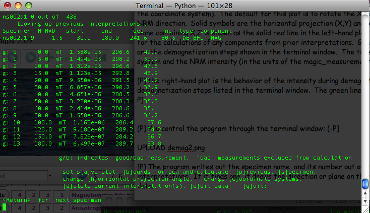
The program writes out the specimen name and its number out of the total, then looks for previous interpretations. If it finds one, it draws the direction or plane on the plot windows and prints out summary data: the specimen name, the number of steps included in the calculation, the MAD or alpha_95 (depending on calculation type), the start and end demagnetization steps, the declination and inclination of the directed line or pole to the best-fit plane, the calculation type (best-fit line, plane or fisher mean or DE-BFL, DE-BFP, DE-FM respectively) and the component name.).
Then, the program prints out the data for the specimen. Each measurement is annotated "g" for good or "b" for bad depending on the measurement_flag in the data file and numbered. The demagnetization level is given in mT or oC. The strength is in SI units and the declination and inclination are in the coordinate system specified in the titles of the plot figures.
The program can be controlled by entering letters on the command line. Hitting the return (or enter) key will step to the next specimen.
When you have stepped through all the specimens, or typed 'q' to quit, the program quits and control is returned to the GUI window. If it seems stuck, click on the python icon on your dock (Macs only) and the GUI will respond again (usually!).
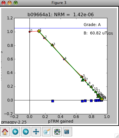
The left-hand plot (labeled Figure 3) is an Arai plot of the double heating experiment. The title is the specimen name and NRM intensity of the specimen. Solid symbols are zero-field first then in-field heating pairs (ZI) data and open symbols are in-field first, then zero field pairs (IZ). The temperature pairs are numbered for reference with the data list in the terminal window. The blue squares are "pTRM-tail checks" and the triangles are "pTRM" checks. If you have selected end points for inclusions in the slope calculation, these will be marked by diamonds and the green line is the best-fit line through the data points. The field intensity will be noted (B: ) in microtesla and a grade assigned according to the selection criteria. To change these, use the "customize criteria" option described above. The line labeled "VDS" is the vector difference sum of the zero field data.
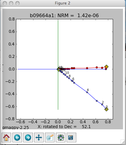
The middle plot is a vector-end point diagram. The magnetization vectors are broken down into X,Y,Z components (these are in specimen coordinates here with the X direction rotated such that it is parallel to the NRM direction. Solid symbols are the horizontal projection (X,Y) and open symbols are the X,Z pairs. The open diamonds are the end points for the calculations of any components from prior interpretations. Green lines are best-fit lines. The numbers are the demagnetization steps shown in the terminal window. The title is the specimen name and the NRM intensity (in the units of the magic_measurements table, so are SI.
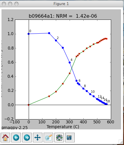
The right-hand plot is the behavior of the intensity during demagnetization and remagnetization. Numbers are the demagnetization steps listed in the terminal window.
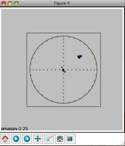
The fourth plot is an equal area projection of the zero field steps from the ZI steps (circles) and the IZ steps (squares) as well as the direction of the pTRM acquired at each step (triangles). This should of course be parallel to the lab field direction and deviation therefrom is a hint that the specimen is anisotropic. Only the steps included in the slope calculation are plotted.
You control the program through the terminal window:
The program writes out the specimen name and its number out of the total, then looks for previous interpretations. If it finds one, it draws the interpretations on the plot windows and prints out summary data: specimen name, lower and upper temperature steps (Tmin, Tmax), the number of steps used in the calculation, N, the lab field assumed, lab_field, the ancient field estimate (no corrections) B_anc and a host of other statistics: b q f(coe) Fvds beta MAD Dang Drats Nptrm Grade R MD% sigma Z Gmax which are described in the Essentials of Paleomagnetism online text book. The program also looks for TRM acquisition data and anisotropy data. If it finds it, it will print out the "corrected data" as well, including the corrected pTRM acquisition steps - a proper anisotropy correction will bring the best-fit line through these into alignment with the laboratory applied field direction. If the program finds TRM aquisition data, there will be a fifth plot, showing these data as well and the correction inferred therefrom.
The program thellier_magic.py can be controlled by entering letters on the command line. Hitting the return (or enter) key will step to the next specimen.
When you have stepped through all the specimens, or typed 'q' to quit, the program quits and control is returned to the GUI window. If it seems stuck, click on the python icon on your dock (Macs only) and the GUI will respond again (usually!). When you are done, be sure to select "Assemble specimens."
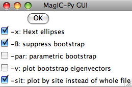
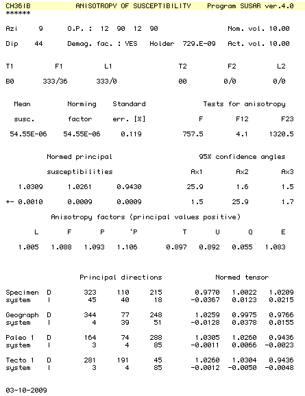
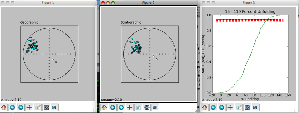
For a complete discussion of confidence ellipses see Chapter 13 in the Web Edition of the book Essentials of Paleomagnetism, by Tauxe et al. (2009). In this example, we elected to plot both the Hext ellipses and the bootstrap ellipses. To suppress the latter, check the box labelled '-B' in the options window. For now, we get this plot:
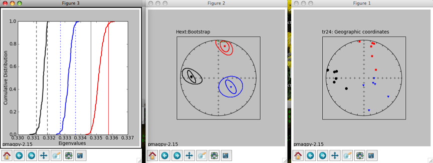
In Figure 1 (to the right), we have plotted the eigenvectors from site tr24. Red squares are the eigenvectors associated with the maximum eigenvalues for each specimen. Blue triangles are the intermediate and black circles are the minima. All plots are lower hemisphere equal area plots. Figure 2 (middle) shows the two forms of confidence ellipses. The rounder, larger ellipses are the Hext ellipses. Green lines are plotted on the upper hemisphere. Figure 3 (left) shows cumulative distributions of bootstrapped eigenvalues and their 95% confidence bounds (vertical lines). Because each eigenvalue is distinct from the others (the confidence bounds do not overlap), this site has a triaxial fabric. These plots can be saved in a variety of formats by clicking on the disk icons to on the figure tool bars by choosing the appropriate name (e.g., myfig.png saves the file in the png format) or by typing an "a" on the command line in the terminal window. [P] [P] To control the program, type in commands on the command line in your terminal window:
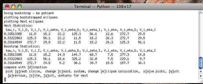
You can change coordinate systems (if you have imported orientation information along with your anisotropy files) by typing a "c", ellipses style, by typing an "e". You can also plot a direction (a lineation observed in the outcrop) or a great circle (the plane of a dike) for comparison. You can also step forward to the next site or back to the previous one. The summary statistics for each ellipse calculation are also printed out in the terminal window. The tau_i are the eigenvalues and the V_i are the eigenvectors. The D's and I's are declinations and inclinations and the zeta and eta are the semi-axes of the major and minor ellipses respectively. These summary statistics calculated by aniso_magic.py are also stored in the file rmag_results.txt in the project MagIC directory.
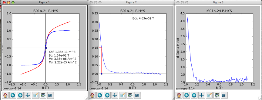
If you also imported data from "back-field" IRM experiments, you will also see a plot like this:
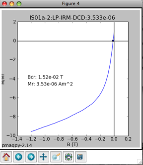
The point at which the remanence is reduced to zero is another estimate for coercivity of remanence. The various hysteresis parameters that are calculated by hysteresis_magic.py are stored in the datafiles rmag_hysteresis and rmag_remanence in the project MagIC directory.
Then, the program steps through the data by site, plotting all the directions in geographic coordinates.
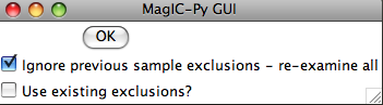
If you find a site with a suspicious sample, you can select 'e' and type in that specimen name on the command line. The program calculates possible specimen directions assuming several common types of errors in the field. Triangle: wrong arrow for drill direction, e.g., out of the outcrop instead of in. Delta: someone read the wrong end of compass. Small circle: wrong mark on sample [cyan upper hemisphere]. Paleomagnetitsts often mark the sample orientation with a brass rod, then extract the sample with a "shoe horn" of some sort. It is possible that when marking the sample, a stray mark was used. In this case, the "real" specimen direction will lie along the dotted line. If any of these possibilities brings the specimen direction into the group of other directions, you can mark this sample orientation as "bad" with a note as to why you have excluded it. The data do not disappear from the data base, but your rationale for excluding a particular result is explained in the er_samples table. The result can be excluded from site means, etc.
When you are done with editing sample orientations, be sure to select "Assemble specimens" again. This will recalculate the specimen tables, excluding the "bad" orientation data from geographic and tilt corrected records.
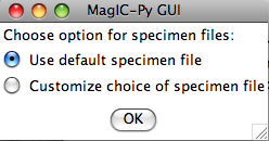
Then you are asked which (of the possibly many) specimen files you wish to work on. The default is the pmag_specimens.txt file generated by the "Assemble specimens" option. If for example, you only want to work on a particular one, select "customize choice". Usually you will want the default specimen file.
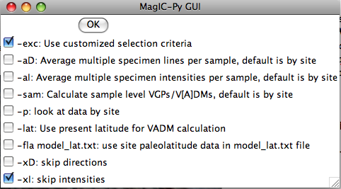
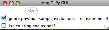
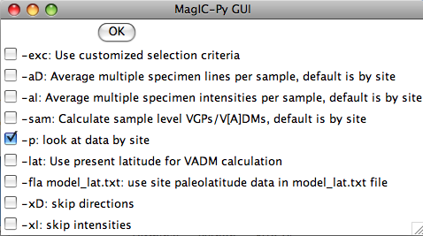
The next window allows you to control which data are selected and how they are treated. To use the selection criteria chosen by you in the "Customize Criteria" section, check the box marked '-exc'. -aD and -aI do the averages by sample, then by site instead of treating all specimens as individuals at the site level. -sam puts sample level VGPs and/or V[A]DMs on the results table. -p plots directions by site so you can have a last check on what is going into the er_sites and pmag_results tables. Virtual Axial Dipole moments (VADM) require an estimate of paleolatitude. This could be the present latitude (-lat option) or a reconstructed paleolatitude (-fla). For the latter, you will have to enter the site name and your best estimate for paleolatitude in a separate file (model_lat.txt). This file should be copied into the project MagIC directory. This latitude will be saved as the model_lat on the results table. If you want to calculate paleolatitudes for a given site, use the "Expected directions/paleolatitudes" option under the Utilities menu. By skipping directions or intensities if you have no relevant data, you can speed up processing time.
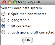
If you have multiple coordinate systems available (e.g., specimen, geographic, tilt corrected), you can choose which coordinate systems you want to include on the pmag_results table:
The specimens_results_magic.py program processes the data, averaging by sample (if desired) and by site. It combines best-fit lines and planes at the site level using the technique of McFadden and McElhinny (1988) and calculates VGPs and V[A]DMs as approprite and creates the files pmag_samples.txt, pmag_sites.txt and pmag_results.txt in the project MagIC directory.
4.3.4 Utilities Menu
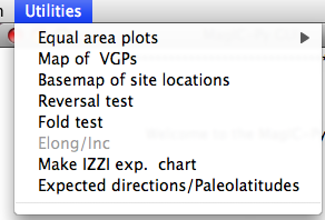
When you pull down the "Utilities" menu, you will see these options:
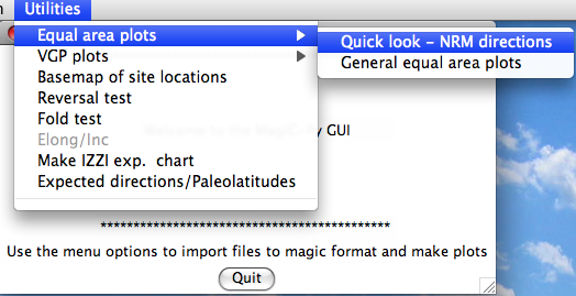
Choosing the "Quick look" option will cause the program to search through the magic_measurements.txt file in your project MagIC directory. The MagIC.py GUI will look into a file called coordinates.txt which is created when you import an orientation file. If you haven't you will only be able to look at the data in specimen coordinates. If you have, you will be asked to specify which coordinate system you desire. Click on the one you want, then on the 'OK' button. You will then see a plot something like this:
The title will specify the coordinate systems. As usual, solid symbols are lower hemisphere projections. In the terminal window, you will see a list of all the specimens that were plotted along with the "method of orientation (SO-) and the declination and inclination found. You can save the plot in the default format (svg) or in some other supported format (e.g., jpg, gif, png, eps) by clicking on the save (the little diskette icon) button on the plot. The default file format can be imported into for example Adobe Illustrator and edited.
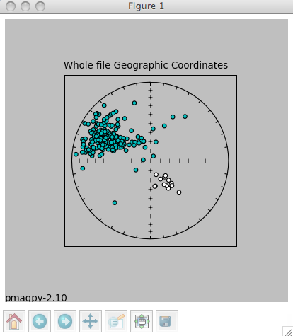
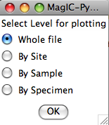
Choosing the general option allows more possibilities, depending on what you have done. You must have selected Assemble Specimens to plot specimen directions or great circles. To plot data for sample or site means, you must first Assemble results. Assuming you have done both, you will be presented with a window that looks something like this:
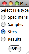
Choose the level you desire by clicking on it, then click on the "OK" button. Next, you must choose which level you want to plot. Be aware that you could choose to plot at the specimen level yet have chosen to look at the site table which has no specimen level data. In that case you would get a message that there were no data to plot. Here we choose to plot the whole file:
Now you can choose what sort of confidence ellipse you want to plot. Fisher statistics, including how to combined lines and planes are explained in Chapter 11 of Tauxe et al., 2009 and the other methods are explained in Chapter 12. Select the method of choice (or None) and click on the "OK" button.
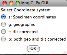
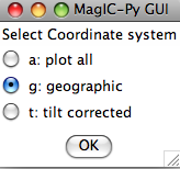
Finally, select your desired coordinate system. You will be presented with a list of options based on what you imported as orientation information. However, if, for example, when you prepared the results file you choose only the geographic coordinate system and not the tilt corrected one, choosing the tilt corrected coordinate system here will result in no data to plot. Here we chose the geographic coordinate system and were presented with this plot:
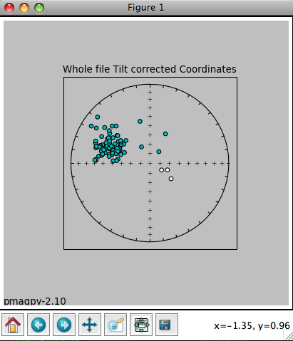
The title reflects the choices that were made. The plot can be saved using the save button or on the command line. In the terminal window you will see a list of the data that were plotted, and the associated method codes. When the eqarea_magic.py program is finished, control will be returned to the MagIC.py
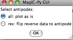
If you choose a coordinate system that is not in the pmag_results.txt file (either because there were no orientation data imported or you did not choose to include it when you assemble the results table), you will have no data to plot. Then you will be asked if you want to flip reverse data to their antipodes. In fact, this option takes all negative latitudes as reverse, so you should be careful with data sets from the Paleozoic or PreCambrian:
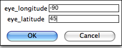
You can customize the projection by setting the position of the "eye". The default is a polar projection.
You will get a plot something like this:
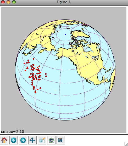
The green square is the spin axis. If you elected to flip 'reverse' data, they will be plotted as green triangles. The plot can be saved in the default format (svg) by typing 'a' on the command line followed by a return (enter) key. For other formats, use the save button on the plot window.
Depending on your choices, you may get a plot like this:
Save the plot by typing 'a' on the command line followed by a return (enter) key, or using the save file button on the plot window itself.
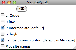
Then it will ask about selection criteria:
And finally, it will give a plot similar to this:
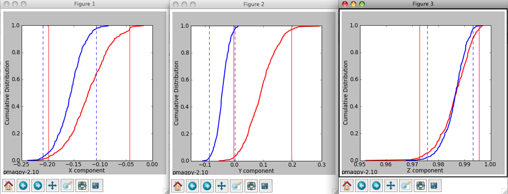
The program takes your data and breaks it into two modes: normal and reverse. It flips the directions in the second mode (usually the reverse one) to their antipodes. Then the program computes the mean direction for each mode and computes the X, Y and Z components for these means directions. Then it re-samples the dataset randomly (a bootstrap pseudo-sample with replacement), generating a new data set which it breaks into two modes, and calculates the components of the mean directions of these. This it repeats 500 times, collecting the components of the two modes. When the bootstrap is finished, the three components of the two modes are sorted and plotted as cumulative distributions in the three plots with the two colors (red for the first mode and blue for the second). The bounds containing 95% of the values get plotted as vertical lines for the two modes. A negative reversals test is achieved when the bounds for the two modes for any of the three components exclude each other.
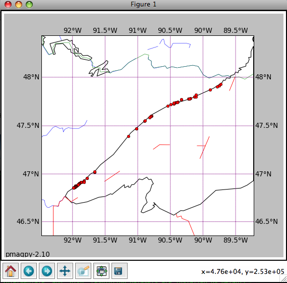
Then the program will generate plots like these:
The left hand plot is of the data in geographic coordinates, the middle is after 100% tilt correction and the right hand plot is a cumulative distribution plot of the maximum eigenvalues obtained through principal component analysis of bootstrapped data after various percentages of untilting. This is a measure of concentration that does not require sorting data out by polarity. The vertical bars are the limits bounding 95% of the data. This particular result is not very impressive allowing peaks in concentration spanning virtually the whole range. The dashed red lines represent the behavior of 20 (out of 1000) bootstrapped data sets.
4.4 Tutorial
4.4.1 Directional Study
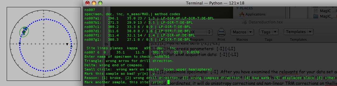
The check orientation option calls the program site_edit.py and steps through the data site by site, printing out sample/specimen information in the terminal window and plotting them, along with the Fisher mean and alpha_95 in the picture window. If a particular directions looks out of place, e.g., ns007b1 in the example data set shown here,
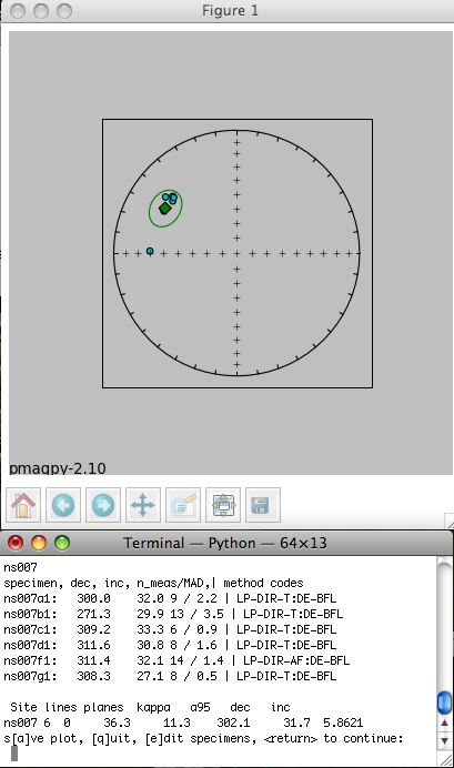
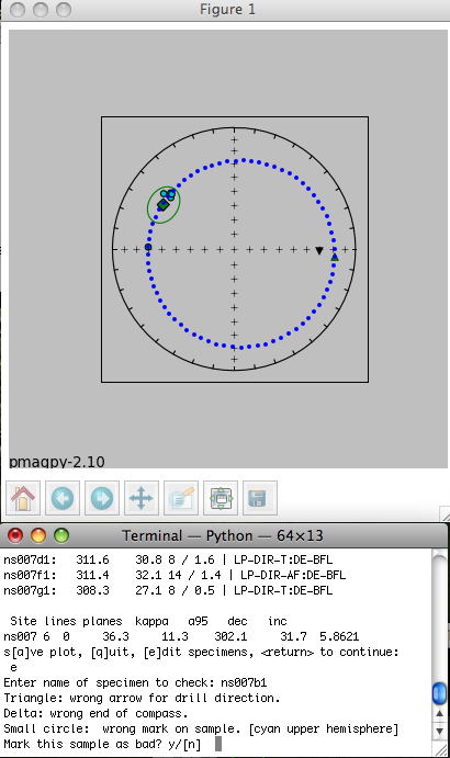
The blue dotted line traces the directions that would be generated if a stray mark on the sample was used instead of the actual drill direction - an interpretation which seems reasonable because the blue dotted line goes right through the directions from all the other specimens at the site. Therefore, type in a 'y' on the command line. And choose "bad mark" as the explanation for rejecting this sample's data. This will mark the sample_flag in the er_samples.txt file as "b" and write in the reason under the sample_description field. Stepping through all the sites allows you to throw out clearly mis-oriented data from your interpretations while preserving the data and the rationale in the database. When the program site_edit.py has finished. You will be asked to run "Assemble Specimens" which is a necessary step before you "Assemble Results". So be sure to choose "Assemble Specimens" from the Import menu before proceeding.
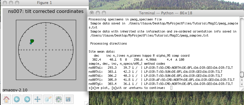
The magic_method_codes summarize how each specimen was treated. The "LP-DIR" method code tells you what type of demagnetization experiment was done (T for thermal, AF for alternating field), the "SO" code tells you about sample orientaion (sun or magnetic compass, for example), the "DE" code documents how the direction estimation was done (BFL for best-fit line or BFP for best-fit plane, for example), the "DA" code lists data adjustments (DIR-GEO, means the data were transformed to geographic coordinates and DIR-TILT means they were also adjusted for tilt). If there is a problem with a site, you can quit the program and return to demagnetization data, or any previous step to track down and fix any problems. If you are satisfied, just step through the sites (there is only one for this tutorial) and the program will finish.
4.4.2 Rock Magnetic Study
Under construction
See also ...
Contents MagIC Chapter 1 Introduction Chapter 2 MagIC Website Chapter 3 MagIC Console Software Chapter 5 MagIC Glossary