ArArCALC Help Library |
|||
|
|
|
||
ArArCALC Help Library |
|||
|
|
|
||
1 Using ArArCALC
The program ArArCALC provides an interactive interface to the data reduction in 40Ar/39Ar geochronology and is coded within Visual Basic for Excel 97-2000-XP using datasheets, charts, menus and dialogboxes. The software is rich in its functionality and contains many utilities that helps you to judge and reduce your age data with more confidence. These utilities fully interact with each other, providing a high level of automation, all within one program and within single age calculation files. In this chapter the basic functionalities are discussed, in order to get you going as quickly as possible with the ArArCALC Software.
1.1 Key Information
Read this section before you install and start to use ArArCALC. In here key information on the User Policy and Development History of ArArCALC are described, as well as how to get Online Help when you are using the ArArCALC Software.
1.1.1 User Policy
ArArCALC is provided as freeware. This software package may be freely used and distributed amongst different research laboratories or educational institutions. The user is only encouraged to exercise proper referencing to the following paper in Computer and Geosciences when publishing data calculated using this software package:
Koppers, A.A.P.
ArArCALC -- Software for 40Ar/39Ar Age Calculations.
Computer and Geosciences 28 (2002) 605-619.
1.1.2 Software and Hardware Requirements
The program ArArCALC is coded in Microsoft Excel 2000/XP/2003 for Windows 95/98/NT/2000/XP. This custom program does not run on Macintosh computers. To run ArArCALC under the Macintosh operating system please install and run VirtualPC first. It is recommended to run ArArCALC on a 2 GHZ computer with at least 512 MB of RAM and a 1024x780 screen resolution.
All program files included with ArArCALC occupy approximately 2.0 MB of total disk space. Typical age calculation workbooks range between 115-500 KB in file size, depending on the number of analyses included.
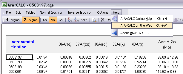
1.1.3 Online with ArArCALC
The ArArCALC Website is continuously maintained at http://earthref.org/tools/ararcalc.htm. You can reach this website by placing a bookmark in your web browser, but you can also select the ArArCALC on the Web (Ctrl+W) menu item from within the ArArCALC software itself. On the ArArCALC Home Page you will find links to the latest downloads and news on the ArArCALC program. The website will be launched in your default browser.
1.1.4 Development of ArArCALC
ArArCALC was initially developed at the Laboratory of Isotope Geology of the Vrije Universiteit in Amsterdam as part of my Ph.D. thesis. In here I like to acknowledge Jan Wijbrans and Gareth Davies for their supportive roles in designing ArArCALC in the early days. The program is currently being maintained and upgraded at the Scripps Institution of Oceanography in La Jolla and since October 2005 ArArCALC is also sponsored through NSF-EAR Instruments and Facilities to further the development of this data reduction package, to make it useful and available to the international 40Ar/39Ar community, and to make it interoperable with the new (still to be developed) online geochronology databases. As a result, I expect that three major upgrades will be brought out over the coming two years.
Please register at EarthRef.org to stay posted on any ArArCALC news or read more on the Future Development Plans. If you have any Requests or Suggestions that will help improve ArArCALC or if you want to share your own Software Code, please contact Anthony Koppers by email.
The first version was programmed already in 1994. Version 1.4 for the Macintosh and version 1.6 for Windows were continuously used as the default data reduction programs at the Vrije Universiteit between 1994 and 1999.
First public release of ArArCALC. The help files are not complete yet but they will be added to the downloadable package on short notice. Macintosh support had to be dropped due to significant incompatibilities in the Macintosh version of Microsoft Excel's Visual Basic for Applications.
Second public release of ArArCALC. This release goes together with the submission of ArArCALC for publication in Computer and GeoSciences. The key functionality of ArArCALC has not changed dramatically, but the following improvements were added and some shortcomings were removed:
Third public release of ArArCALC accompanying publication in Computer and GeoSciences 28 (2002) 605-619. Please Download the ArArCALC paper in PDF format for your own archive and acknowledge the use of ArArCALC by referring to this paper in the Technical Section of your papers. Many improvements were added and some shortcomings were removed. Three highly functional toolboxes have been added (i) to allow for better assessment of the evolution of procedure blanks, (ii) to analyze degassing patterns for all measured argon components, and (iii) to recalibrate the 40Ar/39Ar age calculations all the way back to the primary K-Ar standards. Below follows a short list of the most important updates and changes:
This version of ArArCALC was never released and basically encapsulates a series of intermediate versions of the package, mainly used by the developer himself and by a few beta-testing laboratories. All these improvements are being combined and captured in the release of Version 2.4 in November of 2006.
Version 2.4 -- 22 November 2006
Fourth public release of ArArCALC encapsulating numerous upgrades and bug fixes collated over the last four years. This release marks the first of three major upgrades that will be made public over the coming two years under new funding by the EAR Instrument and Facilities program of NSF. Below follows a short list of the most important updates and changes:
Version 2.5 -- 8 December 2010
Fifth public release of ArArCALC and major overhaul of the underlying code and plotting routines. In addition many new features (see below) have been added and many features have been build in making ArArCALC ready for future enhancements. Below follows a list of the 35 most important updates, improvements and changes:
This intermediate update of ArArCALC was never released and was mainly used by the developer himself to implement a system for bug fixes and small software improvements. It is the intent to release more intermediate versions on a more regular basis.
Version 2.5.2 -- 26 November 2012
First bug fix release of ArArCALC with 14 bug fixes and 4 program enhancements:
1.1.5 Future Development Plans
The ArArCALC software is currently being sponsored through NSF-EAR Instruments and Facilities to further the development of this data reduction package, to make it useful and available to the international 40Ar/39Ar community, and to make it interoperable with the new online GEOCHRON database. The first upgrade already was released as Version 2.4 on 22 November 2006, encapsulating numerous upgrades and bug fixes collated over the last four years. On 8 December 2010 a major overhaul of the software was published as Version 2.5 including 34 bug fixes, improvements and upgrades.
Please register at EarthRef.org to stay posted on any ArArCALC news or return to this page to stay on top of any new Future Development Plans. If you have any Requests or Suggestions that will help improve ArArCALC or if you want to share your own Software Code, please contact Anthony Koppers by email.
1.2 Getting Help
1.2.1 Using Help Files
This ArArCALC package comes with help files written in HTML that are accessible through your web browser. These help files can be reached when running ArArCALC through the Help menu by selecting the ArArCALC Online Help (Ctrl+H) menu item. Note that these help files are not locally stored on your hard drive. This setup allows you to retrieve the most up-to-date help files without downloading the updated help files to your own computer. The ArArCALC Help Library will be launched in your default browser with the Table of Contents as the first page.
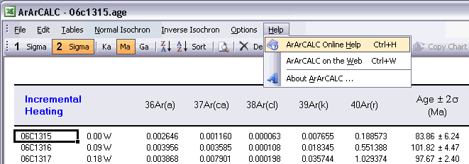
Most dialogboxes used in ArArCALC also have Online Help buttons. Click on these buttons to retrieve "context sensitive help" information from the help files stored in this online ArArCALC Help Library.
1.2.2 Questions and Bug Reports
If you have Questions about ArArCALC or if you want to submit a Bug Report, please contact Anthony Koppers by email. You can also send me your feedback by using the following mailing address or fax number:
When submitting a Bug Report, don't forget to document your problem in as much detail as possible. Describe in which part of the ArArCALC Software you encountered the problem, which function you tried to use, what the error message is, if you come across one, which version of Microsoft Excel you are using, and with which Operating System you are working. It might also be helpful, if you attach one of the *.AGE Calculation Files to your email that showcases the problem.
1.3 Installing and Removing ArArCALC
Installing ArArCALC is not difficult. In this section, the installation process is explained in detail, including how to work with the ArArCALC Log Files, how to install ArArCALC Upgrades, how to install an ArArCALC Icon on your Launchbar, how to Remove the software, and how to deal with the Microsoft Security Settings. Read this section carefully before you start to use ArArCALC for the first time.
1.3.1 Using the ArArCALC.log File
The ArArCALC.log file is the most crucial file while running ArArCALC. In this log file ArArCALC saves all required information with respect to the user-defined Projects, Irradiation Parameters and Calculation Preferences. For this reason, you should make sure to Backup this log file on a regular basis. A backup also needs to be made before re-installing or upgrading ArArCALC. In this way you will not have to re-enter all projects, irradiations and preferences when a newer version of ArArCALC is being copied on top of your current installation.
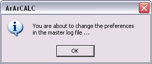
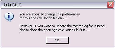
The ArArCALC.log file contains all parameters needed to perform the age calculations that are not already stored in the tables of the age calculation file itself. These parameters range from decay constants to data file locations, irradiation definitions, input filter settings, project definitions, and much more. All these parameters can be viewed and edited via easy-to-use dialogboxes (see also: Managing Irradiations and Projects). When you are going to make changes to the ArArCALC.log file, you always will be warned (see message below) that you're about to change the preferences in the master log file.
Log File Information Attached to *.AGE Files
Since Version 2.4 the Master ArArCALC.log file gets automatically attached to each age calculation file. This happens when creating a new age calculation file, or when you open an age calculation file generated with an older version of ArArCALC. You can also manually re-attach the ArArCALC.log file, if so required (see also: Attach Latest Master Log File).
However, when an age calculation file is already open (and active) in ArArCALC and you want to edit the projects list, irradiation parameters or preferences, the message shown below will appear. This message informs you that your edits will be saved in the age calculation file (and not in the master log file). If you want to edit the Master ArArCALC.log file, you have to close the open age calculation file first.
This setup has important advantages. For example, it allows you to apply specific age calculation preferences on a sample-by-sample basis. It also allows you to send around your age calculation files to colleagues and students, with your user preferences, your irradiation parameters, your formatting and your data selections. This guarantees that the receiving party will see the age calculations exactly as you performed them, when they open your files in ArArCALC. With all your settings now saved in the age calculation files, you also can provide them to publishers to be stored in their electronic archives, as data supplements, or you can store them in the EarthRef.org Digital Archive for long-term online archival.
1.3.2 How to Install ArArCALC on your PC
These are the instructions for installing ArArCALC on your computer:
(1) Copy ArArCALC onto your computer.
(2) Backup crucial ArArCALC files from previous installation.
(3) Set up Microsoft Excel for using ArArCALC.
(4) Define your own irradiations and projects in ArArCALC (see also: Managing Irradiations and Projects).
(5) Define your preferences in ArArCALC (see also: Setting the Preferences).
(6) Now you are ready to reduce your mass spectrometry data (see also: Your First Calculation ... How to Start).
1.3.3 Upgrading ArArCALC
These are instructions for upgrading ArArCALC on your computer:
1.3.4 Removing ArArCALC from your Computer
These are instructions for uninstalling ArArCALC from your computer:
1.3.5 Installing the ArArCALC Icon on the Windows Launchbar
To install an icon of ArArCALC in the Windows Launch Bar as shown below, please follow these instructions:
![]()
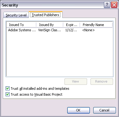
1.3.6 Security Settings
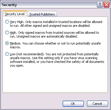
The ArArCALC software uses macros written in Visual Basic for Applications (VBA) for Microsoft Excel. In general, these kind of macros may also provide a security risk, if being used for hacking purposes. To circumvent any risk of opening files that may contain certain malicious software code, Microsoft Excel takes some (default) security measures to protect its users. For example, when you install the Microsoft Excel software for the first time, it does not allow you to open any file that has VBA Macros attached to it, like ArArCALC. In addition, it will not trust (how nice) the Visual Basic Project provided by ArArCALC. So, to enable ArArCALC to run on your computer, follow these instructions:
1.4 Basic ArArCALC Functionality
In this section, the basic steps of ArArCALC are explained, to get you going as quickly as possible. Read this section, in particular, if you're a first-time ArArCALC user. The first part of this section covers How to Start ArArCALC, which Key Settings to define and how to perform Your First Age Calculations. The final part shows you how to Export the age calculations, so that you (or any other user) can read the files directly in Microsoft Excel without running ArArCALC.
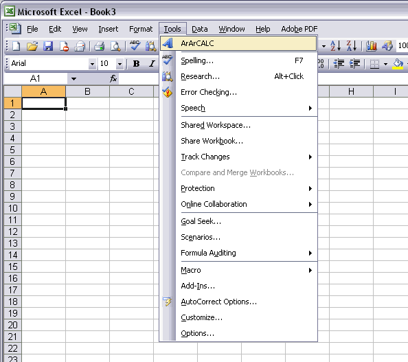
1.4.1 How to start ArArCALC from Excel
ArArCALC is easily launched from Microsoft Excel's Tools menu. Note that ArArCALC saves and closes any file already open in Microsoft Excel. It is assumed that ArArCALC is already installed (see also: How to install ArArCALC on your PC).
Alternatively, you can start ArArCALC from the Windows Launchbar. To activate this functionality please follow the instructions on the Installing the ArArCALC Icon on the Windows Launchbar help page.
![]()
1.4.2 File Organization
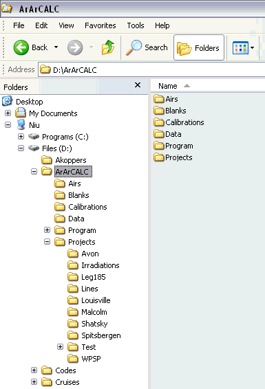
ArArCALC has a simply directory structure with six permanent subdirectories: Airs, Blanks, Calibrations, Data, Program and Projects. Note that in the example below ArArCALC has been installed on the "Files (D:)" drive, but in fact ArArCALC can be installed in any (sub)directory and on any drive available on your local system.
The Microsoft Excel Workbooks containing the age calculations are stored in subdirectories of the Projects directory, which are named according to your project name (see also: Managing Irradiations and Projects). Sub-projects are allowed since ArArCALC Version 2.4 and may result in a directory structure like Projects/OJP/Site 1, Projects/OJP/Site 2, etc. However, it is not advisable to add/delete project subdirectories from within the Windows File Manager or Explorer, before making backups of the Projects directory.
The following files are minimally necessary in the Program directory, when executing ArArCALC:
- ArArCALC.age
- ArArCALC.ico
- ArArCALC.log
- ArArCALC.xla
- ArArCALC.xls
- ArArCALC.xlw
Without these files, ArArCALC will terminate its execution.
1.4.3 File Name Conventions
Starting with ArArCALC Version 2.0 this program does not use a default naming convention anymore. The user will simply be prompted to give in Experiment Name and Sample Type when opening a new mass spectrometry data file (see also: Your First Calculation ... How to Start). This gives the user full control on what type of data is being calculated and under which name the *.AGE files are saved in the Projects directories (see also: File Organization). To collate different measurements for an incremental heating experiment into one and the same *.AGE file always use the same Experiment Name and save the files to the same Project directory.
1.4.4 Managing your Irradiations and Projects
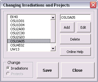
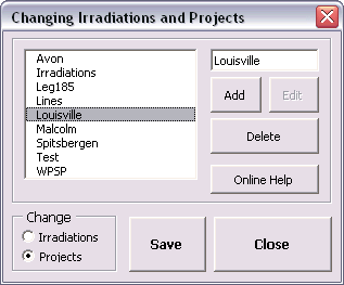
ArArCALC saves all age calculation data files in separate directories according to project name (see also: File Organization). This guarantees an automated and well-structured file organization. However, these project names are logged together with all irradiation parameters in the ArArCALC.log file (see also: Using the ArArCALC.log File). This log file can be accessed and updated through a set of easy-to-use dialogboxes. To activate the Changing Irradiations and Projects dialogbox, select the Options # Irradiation and Projects menu item.
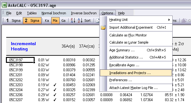
The Changing Irradiations and Projects dialogbox lets you choose what via the option buttons Irradiations and Projects in the lower left Change panel. After making a selection, you can use the Add, Edit and Delete buttons to update either the list of project names or irradiations. To add a new list item, you first need to fill in the name of a new irradiation or project in the textbox in the upper right corner, followed by clicking the Add button. To edit or delete an existing irradiation or project, you first click on its name in the list box, followed by clicking either the Edit or Delete button.
If you want to save your edits, please hit the Save button first, because the Close button will close the Changing Irradiations and Projects dialogbox without saving. If you want to ignore or undo any of your changes, hit the Close button without hitting the Save button first.
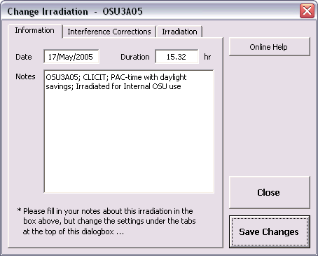
When adding or editing irradiation definitions, ArArCALC will show you the Change Irradiation dialogbox to allow you to define the irradiation parameters, including up to 999 irradiation segments or cycli (see further below).
information
In this tab you can find summary info and notes for a particular irradiation. In here only the Notes can be edited and it is highly recommended that you provide a short description of the irradiation in this field. This description may include which reactor was
used, whether the samples were shielded or not, the purpose of the irradiation, the related project(s) and what time zone was used in the definition of
the Irradiation Cycli or Segments (see below). The Date and Total Duration of the irradiation are automatically calculated from the Irradiation Cycli
data, where the Date represents the first segment listed in the irradiation list and the Total Duration the summed durations as listed in the first column.
Interference Correction
In this tab you should define the Interference Correction factors and their uncertainties. These constants differ per reactor and whether the samples were shielded or not.
Irradiation segments
In the final tab you can define the Duration, Date, End Time and MW (reactor power) of all Irradiation Cycli or Segments.
It is highly recommended that you use either GMT or your Local Time Zone, as long
as you consistently apply it throughout ArArCALC. For example, you should make certain that you apply the same Time Zone when you define your irradiations and when you supply dates and times in the
Sample Parameters
(see also: Sample Parameters). Use the spin button to increase or decrease the Number of Irradiation Segments. Click on a line in the list box to adjust your settings, which will appear for editing in the
text boxes at the bottom of this dialogbox. To speed up data entry you can also check the Auto Fill option.
1.4.5 Setting your Preferences and Input Filters
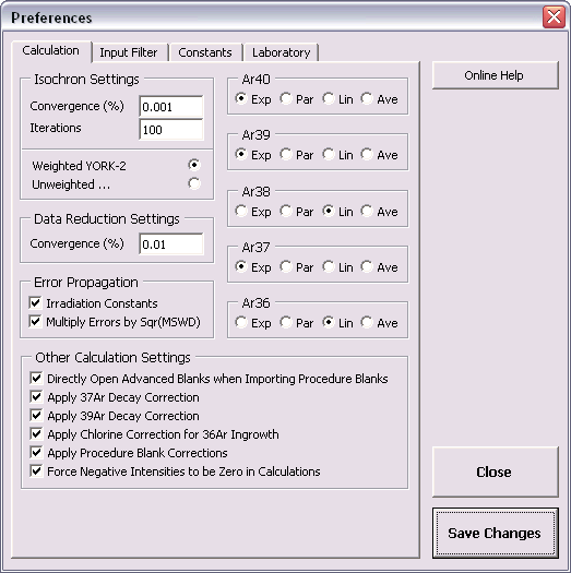
The program ArArCALC does not contain any constant in its computer code. Every constant, parameter and setting can be set by the user. This is done to give you 100% control over what you calculate in ArArCALC. Below follows a list of adjustable settings in the Preferences dialogbox.
Isochron Settings
These options let you influence the precision of the YORK2 Isochron calculations (see reference: York, 1969). The Convergence determines how small the difference in slope of the isochron should be for two consecutive iterations to result in a successful least-squared fit. The
Convergence is here expressed as a percentage of the slope itself (see also: Isochron Calculations). The number of Iterations determines after how many iterations the isochron calculation should
be terminated, in case the calculation is not converging. If you set the Convergence to a higher precision (a lower percentage),
you also should adjust the number of Iterations accordingly (to a higher number). Clicking the option button Weighted YORK-2 forces ArArCALC to calculate a least-squared linear fit with correlated errors that is weighted by the inverse of the variance (see
reference: York, 1969). You can overrule this setting when performing isochron calculations by selecting
Normal Isochron # Weighted YORK-2
or Normal Isochron # Unweighted YORK-2 in the menu bar.
You can do the same for the Inverse Isochron independently.
Data Reduction Settings
The data reduction settings determine the precision when you apply the Exponential
Fit to your mass spectrometry data. The Convergence is expressed as a percentage of the curvature coefficient that is iteratively derived in this least-squared fit (see also: Line Fitting).
Error Propagation
By checking Irradiation Constants in the Error Propagation box, the errors on the
irradiation correction factors will be propagated in the reported analytical error (see also: Analytical, Internal and External Errors). You can set these errors in the Change Irradiation dialogbox (see also:
Managing Irradiations and Projects). If the Multiply Errors by Sqr(MSWD) is checked, then the errors on the ages and some isotope ratios (e.g. 40Ar/36Ar and 40Ar/39Ar)
will be multiplied by the sqr(MSWD) in case the MSWD becomes larger than 1 (see also: Analytical, Internal and External Errors). Both options are activated by default in ArArCALC.
Ar40, Ar39, Ar38, Ar37 and Ar36
You can chance the option buttons to the right of the Preferences dialogbox in order to set your Default Calculation Type for the raw data reductions
(see also: Line Fitting). You can do this independently for each isotope by choosing from four calculation types: exponentional (Exp), parabolic or second order
polynomial (Par), linear (Lin) and averaging (Ave). You can always overrule these default settings in ArArCALC when performing the actual line
fits.
Other Calculation Settings
With
these checkboxes you can determine which Additional Corrections to apply (or not apply) during the age calculations (see also: Other Calculation Settings). However, it is always recommended that you apply
the corrections for 37Ar and
39Ar Decay following sample irradiation, for
36Ar Ingrowth in chlorine-rich samples, and for Procedure Blanks.
However, for samples younger than 1 Ma it is recommended that you uncheck the Force Negative Intensities to be Zero
... option. This will allow for more accurate age calculations, because
negative ages (or error bars) are statistically expected and valid for these
kind of samples. ArArCALC will generate a
warning when you select a non-default setting.
Defining your own Input Filter is most critical while using ArArCALC. Although it may look complicated, it gives you the flexibility to read-in different types of mass spectrometry data files. ArArCALC does not read-in binary files and expects that the measurements were saved in sequentional text files. Furthermore, the actual intensity measurements should be given per line, including the intensity (in volts, amps or counts) and the time (in hours, minutes or seconds) after inlet of the argon gas in the mass spectrometer. By clicking on the Settings button you can define the internal structure of both the header and data sections in a separate dialogbox (see explanation below). By checking the Choose Input Filter when ... checkbox, ArArCALC allows for the selection of an input filter every time you open a new data file. Otherwise the input filter selected in the list box shown below will be used by default.
General Settings
The File Structure is determined by the Number of Header Rows and the Number of Peak Measurements for each measurement cycle, and whether the
text file is Space, Comma or Tab delimited. The Number of Peaks should be at least five to cover all five argon peaks between Ar36
and Ar40. In the Peak Cycle Structure the user defines which lines represent
peak measurements for the argon isotopes and which lines represent baseline measurements. These lines can be assigned in random order as long as the Number of Peaks is not exceeded.
If you provide two baseline measurements, ArArCALC calculates an average baseline (see Ar36 through Ar39 below). If you provide one baseline measurement, the baseline value will be
subtracted as is (see Ar40 below). You can also fill in "0" when your data already have been baseline corrected (by your data acquisition software, for example). Two positions for the masses
Ar41 and Ar35
have already been reserved for future importing and monitoring of this data.
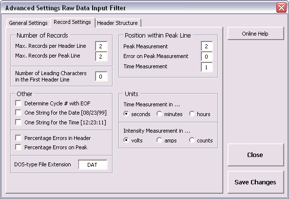
Record Settings
In the
Record Settings tab you can define which records in the peak lines represent the Peak Measurement, the Error on Peak Measurement and the Time Measurement.
Here you can also define in which units the Time
and Intensity Measurements are given and you can define settings such as
the File Extension, the Maximum Number of Records and Header Lines, and how the Date and Time parameters
and the Errors are represented in the
data files. By default
ArArCALC assumes absolute errors.

Header Structure
Your raw data files may contain more than 1 header line. In the
Header Structure
tab you can define on which header line (H#) and on which record position (R#) the Sample Name or J-Value was stored. This of
course requires that these headers were originally saved in the data file. In the rather simple example below, only one parameter is stored, namely the Number of Cycli, which is stored in the first record of the first header line. Further below a more
complicated example is shown and explained as well.
Example 1 Space delimited text file 1 header line; 10 peak measurements | |
10 5.76734625000000E-0000 9.06800000000003E+0001 3.50166666666667E-0003 1.01855000000000E+0002 1.61403125000000E-0001 1.18145000000000E+0002 3.44500000000000E-0003 1.33135000000000E+0002 6.75000000000000E-0003 1.43025000000000E+0002 3.48000000000000E-0003 1.52855000000000E+0002 3.16950000000000E-0002 1.62740000000002E+0002 3.45666666666667E-0003 1.73865000000002E+0002 1.01312500000000E-0002 1.90145000000000E+0002 3.39500000000000E-0003 2.06435000000001E+0002 5.64673875000000E-0000 2.17610000000001E+0002 3.51833333333333E-0003 2.28845000000001E+0002 1.60882500000000E-0001 2.45105000000000E+0002 3.44000000000000E-0003 2.60125000000000E+0002 6.74500000000000E-0003 2.70010000000000E+0002 3.56250000000000E-0003 2.79840000000000E+0002 etc. etc. |
The number of cycles Cycle 01; Line 01 = mass 40.0; time in seconds Cycle 01; Line 02 = mass 39.5; time in seconds Cycle 01; Line 03 = mass 39.0; time in seconds Cycle 01; Line 04 = mass 38.5; time in seconds Cycle 01; Line 05 = mass 38.0; time in seconds Cycle 01; Line 06 = mass 37.5; time in seconds Cycle 01; Line 07 = mass 37.0; time in seconds Cycle 01; Line 08 = mass 36.5; time in seconds Cycle 01; Line 09 = mass 36.0; time in seconds Cycle 01; Line 10 = mass 35.5; time in seconds Cycle 02; Line 01 = mass 40.0; time in seconds Cycle 02; Line 02 = mass 39.5; time in seconds Cycle 02; Line 03 = mass 39.0; time in seconds Cycle 02; Line 04 = mass 38.5; time in seconds Cycle 02; Line 05 = mass 38.0; time in seconds Cycle 02; Line 06 = mass 37.5; time in seconds etc. etc. |
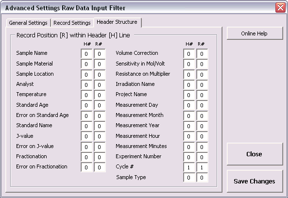
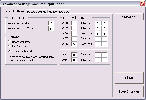
This is one of the most simple text files possible (see settings in the dialogboxes displayed above). Its space delimited and it has the minimum amount of headers. The Number of Headers should be set to 1 and consequently the Cycle # should be set to [1,1] as well. Since there is only one header line with only one parameter in it, all other possible header positions should be set to zeros (which is the default value). In this example, each measurement cycle produces 10 individual peak measurements (5 isotopic peaks and 5 baselines) and thus the Number of Peaks should be set at 10. The net peak of Ar40 is calculated based on peak 1 minus the average baseline calculated from peak 2 and peak 2, the net peak of Ar39 is calculated based on peak 3 minus the average baseline calculated from peak 2 and peak 4, etc. etc.
Example 2 Comma delimited text file 10 header lines; 6 peak measurements | |
98Haw001 Plagioclase Deep Canyon Anthony Koppers 1100 0.000345,0.3 1.00038,5.7 VU13 12 19-Mar-1999,14:34:03 5.76734625000000E-0000,9.06800000000003E+0001 1.61403125000000E-0001,1.18145000000000E+0002 6.75000000000000E-0003,1.43025000000000E+0002 3.16950000000000E-0002,1.62740000000002E+0002 1.01312500000000E-0002,1.90145000000000E+0002 3.39500000000000E-0003,2.06435000000001E+0002 5.64673875000000E-0000,2.17610000000001E+0002 1.60882500000000E-0001,2.45105000000000E+0002 6.74500000000000E-0003,2.70010000000000E+0002 etc. etc. |
Sample Name Material Location Analyst Temperature J-value and %SD Fractionation correction factor and %SD Irradiation Name The number of cycles Measurement date and time Cycle 01; Line 01 = mass 40.0; time in seconds Cycle 01; Line 02 = mass 39.0; time in seconds Cycle 01; Line 03 = mass 38.0; time in seconds Cycle 01; Line 04 = mass 37.0; time in seconds Cycle 01; Line 05 = mass 36.0; time in seconds Cycle 01; Line 06 = mass 35.5; time in seconds Cycle 02; Line 01 = mass 40.0; time in seconds Cycle 02; Line 02 = mass 39.0; time in seconds Cycle 02; Line 03 = mass 38.0; time in seconds etc. etc. |
This is a more complicated text file that can be read-in by ArArCALC (see settings in the dialogboxes displayed below). Its comma delimited. It has 10 header lines as is set for the Number of Headers. Each measurement cycle produces 6 individual peak measurements (5 isotopic peaks and 1 baseline at mass 35.5), explaining why the Number of Peaks is only set to 6. The net peak of Ar40 is calculated based on peak 1 minus the average baseline calculated from peak 6 and peak 6 (which is the actual baseline value as measured on mass 35.5), the net peak of Ar39 is calculated based on peak 3 minus the average baseline calculated from peak 6 and peak 6, etc. etc.
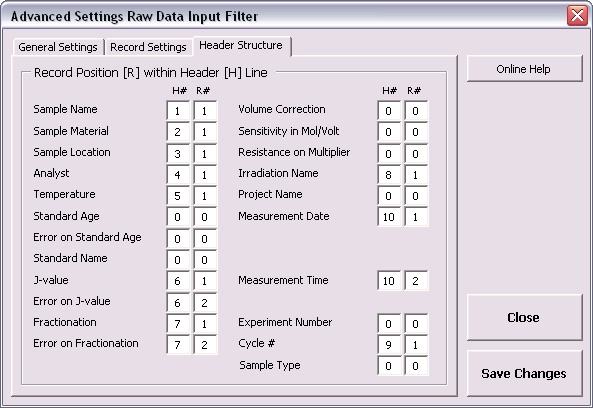
The number of cycles can be found on the first record of the 9th header line in this text file and the Cycle # is thus set to [9,1]. The Sample Name, Material, Location and Analyst are all located on the first record of header lines 1 through 4. The Temperature for the measurement is located on header line 5, the J-value and Fractionation Correction Factors and their errors are located on header lines 6 and 7 at records 1 and 2, respectively. The Irradiation Name is located on the first record of header line 8. Finally, the Date and Time are located on header line 10 at records 1 and 2 as well. Since the One String for the Data and Time checkboxes have been selected (see above) only one option is available to you for the Date and Time. If you have them unchecked, you can point to individual values for the Day, Month, Year, Hours and Minutes in the header structure.
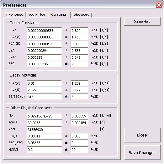
The Decay Constants and their percentual standard deviations can be set and changed in the Preferences dialogbox below. Here you can also define the data for Decay Activities and Other Physical Constants that are needed for the primary age calculations and recalibrations based on the formulations of Karner & Renne (1998), Renne et al. (1998) and Min et al. (2000). For more details read the Primary Age Recalibration Toolbox help page. The expected units are given in the brackets, unless the numbers are dimensionless.
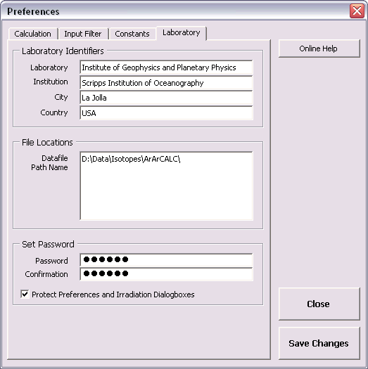
The information you fill out in the Laboratory Identifiers panel will always be printed as headers and footers, next to the date, time and the ArArCALC version number, when you are making a printout from within ArArCALC. You can also set the File Location of the mass spectrometry data files on your hard disk to ensure that ArArCALC swiftly finds your data files. Finally, you may want to set a Password to protect your settings in the Preferences and Irradiation and Project dialogboxes. Setting passwords is, in particular, advised for the person who is managing the Master ArArCALC.log file, in order to circumvent accidental deletion of these important parameters (see also: Using the ArArCALC.log File).
1.4.6 Your First Calculations
Let's assume that ArArCALC is already running (see also: How to start ArArCALC from Excel) and that you have already set your own Project names, Irradiation
Parameters and Preferences (see also:
Managing Irradiations and Projects, Setting the Preferences). Now you are ready to do your first calculation.
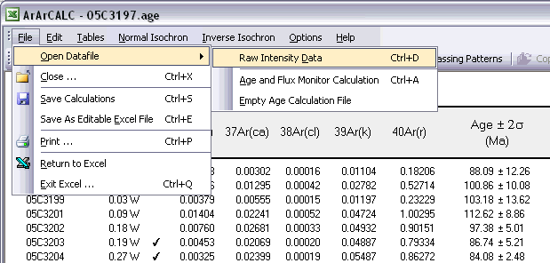
Open a raw intensities data file by selecting the File # Open Datafile # Raw Intensity Data menu item.
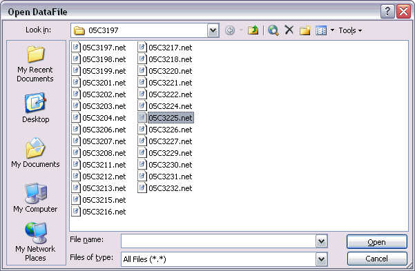
This will give you the following Open DataFile dialogbox. You can set the default file location for these type of data files in the Preferences dialogbox (see: Setting the Preferences) to speed up your file search. Now scroll, select and Open your data file.
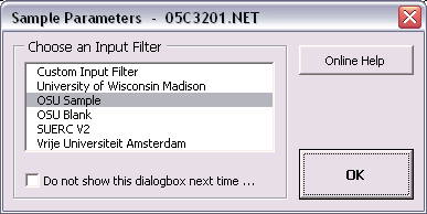
When you open your data file, ArArCALC will show you three dialogboxes in sequence. In the first dialogbox, you have to select an Input Filter. However, you can surpass this dialogbox by unchecking the Choose Input Filter when ... checkbox in the Preferences (see: Setting the Preferences) or by checking the Do not show this dialogbox ... checkbox in the dialogbox shown below. You can use the latter option when you always open your data files with the same input filter.
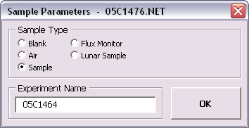
In the second dialogbox, you have to set the Sample Type and give an Experiment Name (See also: File Name Conventions, Sample Type and Experiment Name). When you choose a Blank as the sample type, however, the experiment name is not necessary and thus will be grayed out. To collate different measurements (from different data files) for an incremental heating experiment into one and the same age calculation file, always use the same Experiment Name and save the files to the same Project directory (see next step).

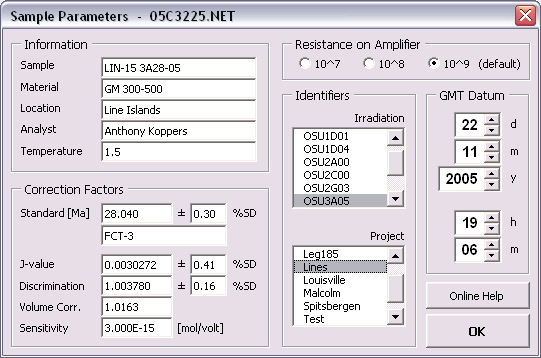
In the final dialogbox, you have to set all Sample Parameters necessary to perform an age calculation. The shown fields are always pre-filled with data from the previous calculation, even if these were performed a few days or weeks ago. Completing this dialogbox will be fast, because most entries will be similar and thus don't need changing when regression data from a single (incremental heating) experiment. Most likely, only the GMT datum and Temperature need editing, unless you start to reduce a totally new experiment. If your raw data files already have header lines containing this information, ArArCALC will automatically transfer this header information into this dialogbox by using your Input Filter (see also: Setting the Preferences). Even in this highly-automated setup this dialogbox will be useful to you, because it allows you to check and edit the sample parameters before further processing of the data commences. You can always recall this dialogbox at a later stage in the Raw Data Reduction view of ArArCALC via the Options # Sample Parameters menu in order to edit the sample parameters.
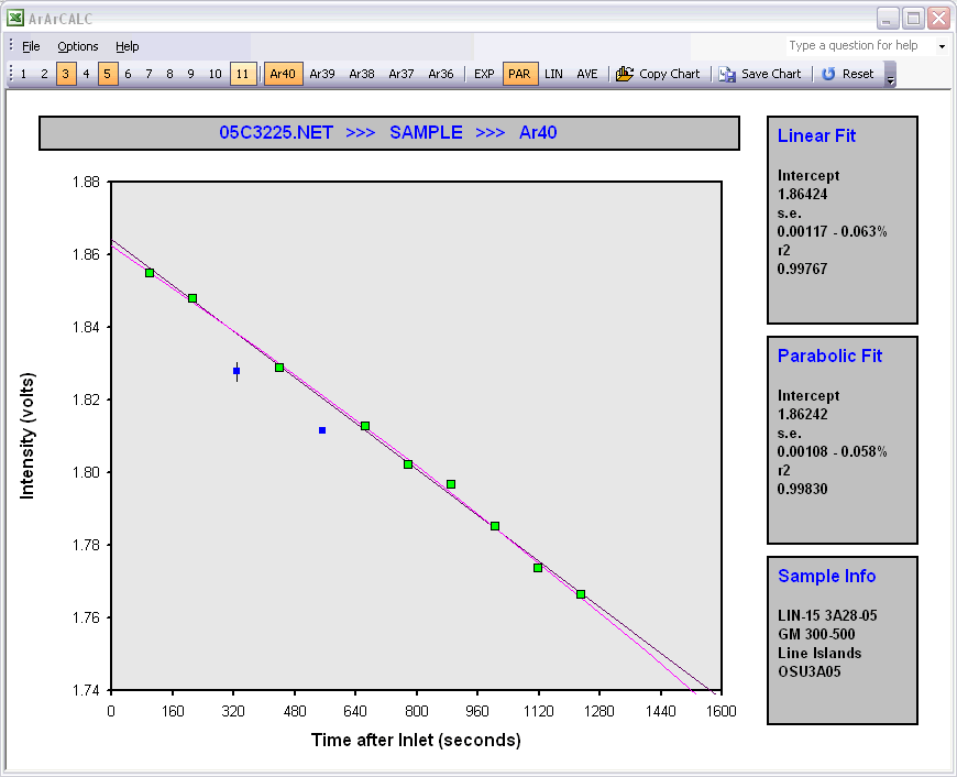
If you have entered all the sample parameters, you will be guided to the Raw Data Reduction view. In this view, a XY-scatter plot displays the measurement time (in seconds) after the inlet of the argon sample in the mass spectrometer on the X-axis, and the intensity of the beam on the Y-axis (in volts, amps or counts). By default, the intensity data for Ar40 is shown first. Each different argon isotope can be calculated by clicking the isotope buttons Ar40, Ar39 ... Ar36. Data points can be included or excluded from the calculations by clicking the toolbar buttons 1, 2, 3, 4 ... 11 that represent the data points, or by clicking the data points themselves on the diagram. Excluded data points are denoted by blue squares and a suppressed toolbar button. The Reset button recalculates including all data points. ArArCALC does not decide which fit to the data (exponentional, parabolic, linear or average) gives the best results. For this purpose, you can set the default regression type for each argon isotope in the preferences (see also: Setting the Preferences). Only in one particular case, when the exponential and parabolic are similar to the linear least-squared fit, ArArCALC accepts a linear fit by default. However, based on the calculation results (see the boxes to the right of the scatter plot) you can always overrule these program decisions yourself, by choosing the appropriate button on the ArArCALC toolbar: Exp, Par, Lin or Ave.
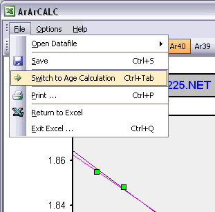
ArArCALC saves all calculated argon intensities of one experiment in one Microsoft Excel 2000-XP-2003 workbook that includes two plateau diagrams and two isochron diagrams, and their respective data tables. The connection between the Raw Data Reduction view (see above) and the Age Calculation view of ArArCALC is easily made through the File # Switch to menu bar item (see also: Switch to ... Option). When you select this option, ArArCALC first saves the calculations and then switches to the age calculation view. You can also make this switch without saving the calculation, by holding down the SHIFT key. If you do not want to switch yet, but you would like to reduce another raw data file, first choose File # Save to save the calculation and then choose File # Open Datafile # Raw Intensity Data to open a new data file.
The following data table will be shown in ArArCALC when you switch to the Age Calculation view. In the shown data table, single incremental heating steps can be excluded or included from the age calculation by double-clicking on the Check Mark symbols. This will automatically recalculate the weighted means, isochrons and other statistics. The Reset button recalculates including all data points. In ArArCALC all errors are calculated as 1 Sigma or 2 Sigma errors. You can report the ages in either the Ka, Ma or Ga age units.
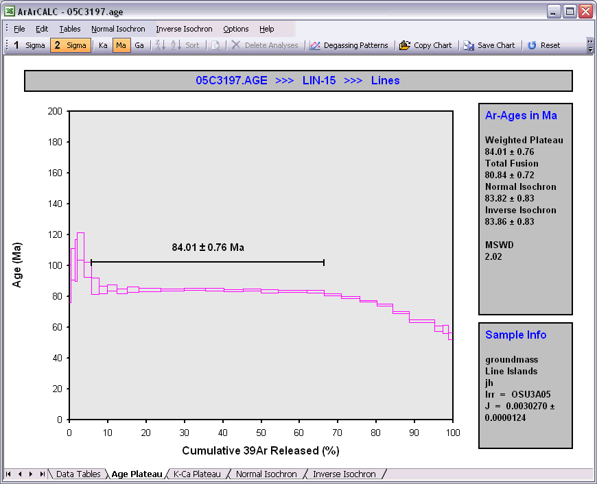
Maneuvering between the different data tables (see also: Selecting Different Data Tables in ArArCALC) and diagrams is simply achieved by clicking the worksheet tabs Data Tables, Age Plateau, K-Ca Plateau, Normal Isochron or Inverse Isochron. Below an example is given for a typical age plateau diagram.
Performing data reductions for Blank and Air Shot measurements starts off the same as for all other measurements. Therefore, the same instructions, as described above, should be followed. ArArCALC saves all reduced blank and air measurements in text files organized per measurement date (blank) or experiment name (air). These files are always stored in the ArArCALC/Blanks and ArArCALC/Airs directories.
1.4.7 Open your Age Calculation in Excel without ArArCALC
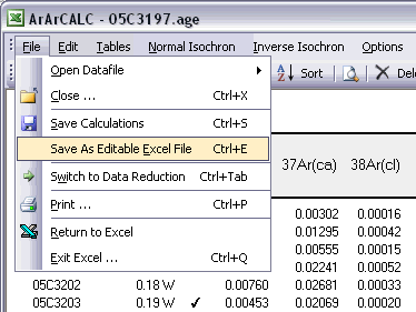
The standard Age Calculation workbooks with the extension *.AGE cannot be opened in Microsoft Excel 2000-XP-2003 without running ArArCALC. These files are password protected to circumvent the possibility of (unexpected) changes made to the workbooks, leaving these files unreadable by ArArCALC itself. However, if you save your calculations via the File # Save as Editable Excel File (Ctrl+E) option, the password protection and the Microsoft Excel macros are removed. Now you can open these newly-saved files with the extension *.XLS in Microsoft Excel and change the format of their data tables and diagrams manually. A progress bar appears, showing you the status while saving these editable files.
1.5 Navigating and Flagging Data Points
ArArCALC is a visual tool that allows you to perform all functions with your Mouse, but also has many Keyboard Shortcuts that allow you to quickly activate certain functions. In this section, it is explained how to Navigate between the tables in your age calculation files, how to use your mouse in Flagging your analyses, and how to Delete your analyses, if so required.
1.5.1 Switch to ... Option
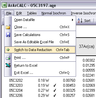
Switching from the Raw Data Reduction view to the Age Calculation view while saving your calculations is very simple. To do so, you should select the File # Switch to Age Calculation (Ctrl+Tab) menu option. Your calculations will be automatically saved (see also: Saving Data Reductions) and, if not possible, you will be notified with a warning. This functionality allows you to reduce your argon mass spectrometry data and then directly switch to the age calculations to check on the results. During this switching you can always suppress the saving, if you hold down the SHIFT key.
Switching from the Age Calculation view to the Raw Data Reduction view is very simple. To do so, you should select the File # Switch to Data Reduction (Ctrl+Tab) menu option.
1.5.2 Selecting Calculation Data Tables in ArArCALC
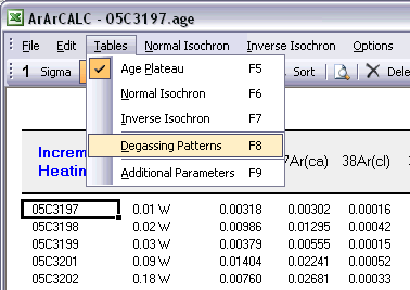
Nine different data tables are available in every ArArCALC age calculation file. Five of these tables include output data from your age calculations, whereas four tables include the input data necessary to perform the age calculations and which you can edit at any time (see also: Editing Data in ArArCALC). The calculation data tables are all located in the Data Tables worksheet and are selectable through the Tables menu. You can also use the F5, F6, F7, F8 and F9 keyboard strokes for faster navigation between the tables.
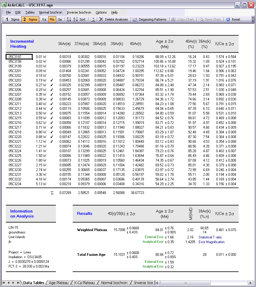
The Age Plateau data table contains calculation data for the plateau age, total fusion ages and K/Ca ratios. Note that also the MSWD, the number of increments and the total amount of 39Ar(k) in percent are given for the age plateau calculation. The uncertainties on the 40Ar/39Ar ages are defined as Internal Errors that combine the Analytical Errors with the Errors on the J-value. For completeness, the Analytical Errors and External Errors (including the error on the total 40Ar decay constant) are given as well (see also: Analytical, Internal and External Errors). The checkmarks signify the analyses included in the age plateau calculation, whereas the summed 36Ar(a), 37Ar(ca), 38Ar(cl), 39Ar(k) and 40Ar(r) components at the bottom of the table are used to calculate the total fusion (or recombined) age.
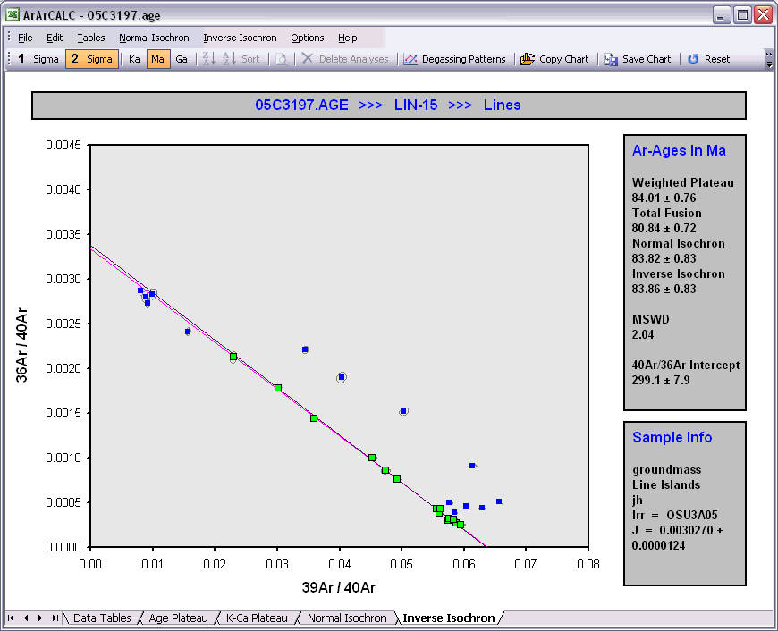
The Normal Isochron and Inverse Isochron data tables contain the calculated ratios 39Ar/36Ar, 40Ar/36Ar, 39Ar/40Ar and 36Ar/40Ar as used in the York (1969) isochron calculations. Both tables display correlation coefficients (r.i) denoting to what extend the errors used in these isotope ratios are correlated. In the example of an inverse isochron below, the correlation is minimal, because the error in the 40Ar (denominator) is small compared to the errors on 39Ar and 36Ar (the nominators). In the Statistics section the isochron calculations are further described by the convergence, number of iterations, type of calculated line, F-ratio, error magnification factor, and the number of points included in these calculations.
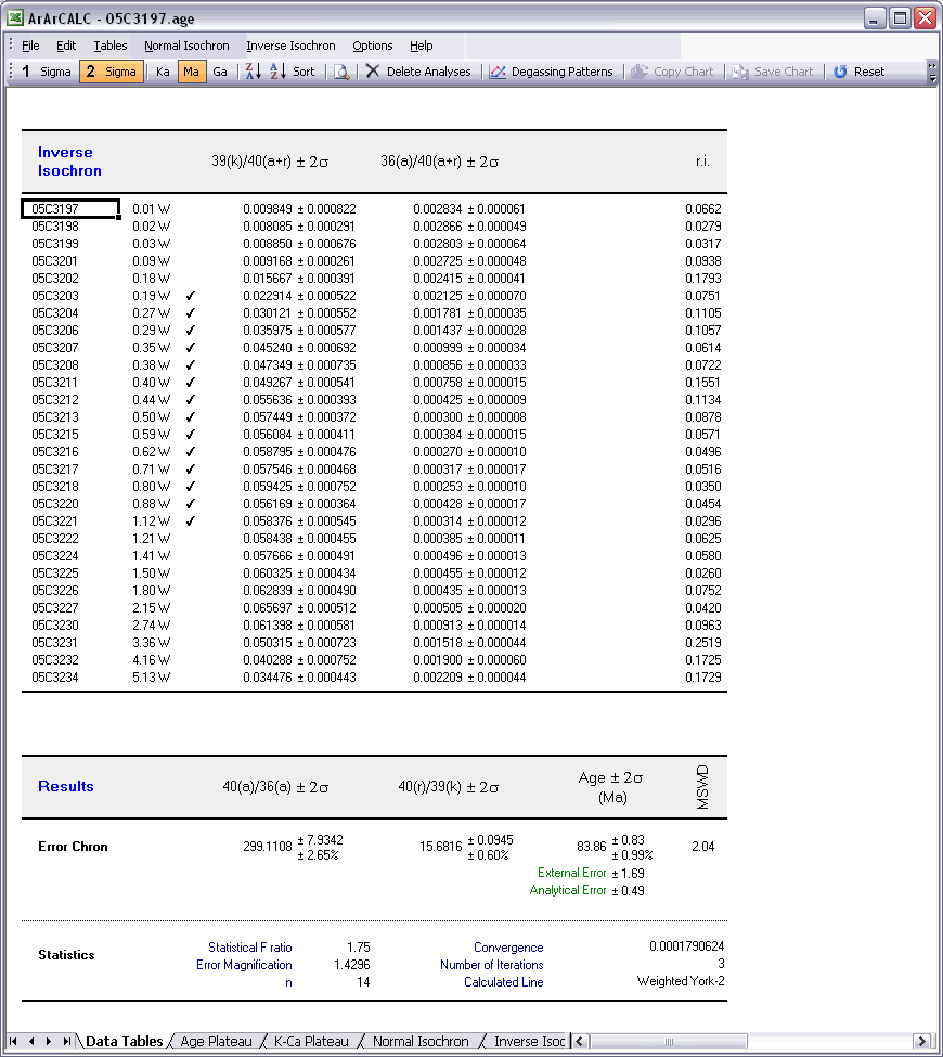
The Degassing Patterns data table contains for every analyses in your experiments the calculated argon components. For example, the entire measurement for the 36Ar isotope can be divided into the 36Ar(a) atmospheric, 36Ar(ca) calcium and 36Ar(cl) chlorine components, and if you are analyzing lunar rocks, also the 36Ar(c) cosmogenic component. For each individual component all increments or steps are summed, while the components themselves are summed as well (see the bottom of the table). A selection of these summed components appears in the Age Plateau data table as well (see above) and they are used to calculate the total fusion ages or to display these in the isochron diagrams (see also: Total Fusion Points in Isochron Diagrams). You can also visualize the Degassing Patterns in an interactive toolbox (see also: Degassing Patterns Toolbox).
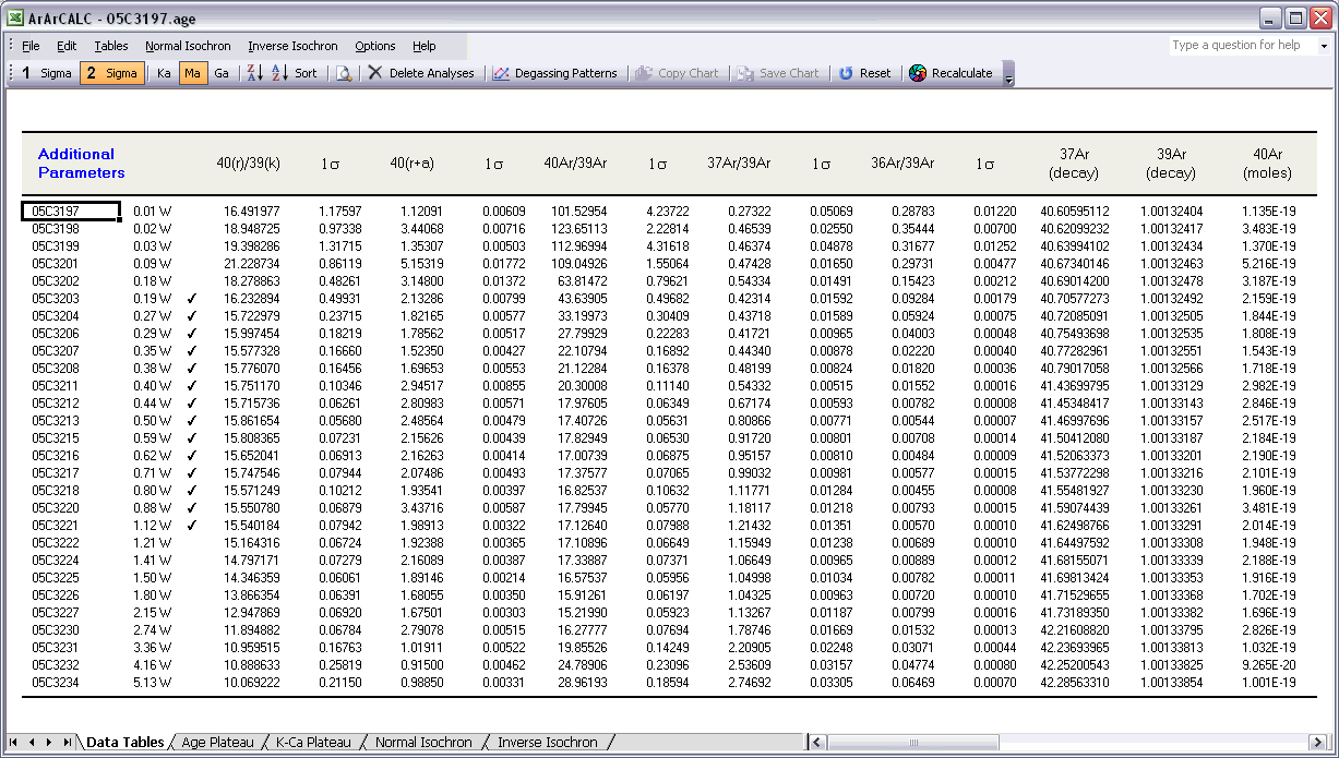
The last data table for Additional Parameters contains an extra selection of data that may be interesting to you when judging the outcome of your argon experiments. Most notable are the decay correction factors for 37Ar and 39Ar, which are used to correct for radioactive decay occurring between the irradiation of the sample and your actual measurements. But also the absolute amount of 40Ar measured is listed here in moles, and the corrected 40Ar/39Ar, 37Ar/39Ar and 36Ar/39Ar ratios and their uncertainties.
1.5.3 Editing Data in ArArCALC
Four data tables in ArArCALC include data necessary for the age calculations, but which you always can edit. These data tables are all located in the Data Tables worksheet and can be selected through the Edit menu. You can also use the F1, F2, F3 and F4 keyboard strokes for faster navigation between these tables.
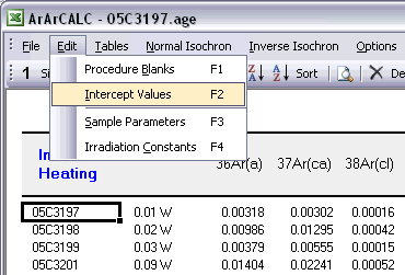
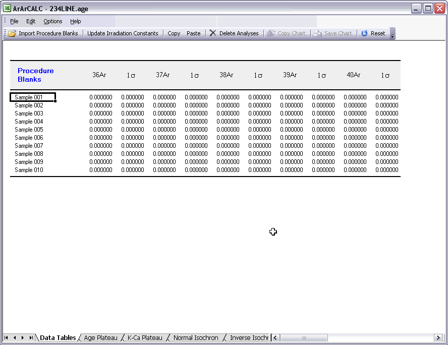
ArArCALC has been set-up to run on-line during mass spectrometry and by default uses the latest-calculated blank measurement for its blank corrections. However, you can always edit the blank intensities later via the Edit # Procedure Blanks menu item. This function displays a data table containing Blank Intensities and their 1σ Standard Error (SE) for each analysis (step) in your (incremental heating) experiment. You can edit these blank data by clicking the cells and typing in new values. A single click lets you replace the complete number, whereas double-clicking will allow you to edit the number within its cell. To copy values from one cell to another, use the Drag functions of Microsoft Excel (drag the black square anchor visible on the highlighted cell down or to the right) or use the Copy (Ctrl+C) and Paste (Ctrl+P) buttons. Note that you can also copy blank values via the clipboard, in which case you select the cells in which to place your new values and use the Paste (Ctrl+P) button. The Reset button will undo all edits, unless you already have saved them.
You can also select single (or multiple) cells, representing one (or more) analyses, and then choose Import Procedure Blanks from the toolbar. Since ArArCALC saves all blank measurements in text files organized per measurement date, this function allows you to import multiple blank measurements for a range of days, by opening more than one of these text files. Blank measurements can now be selected in the Select Blank Files list box to calculate Average Blanks for all argon isotopes, including their (predicted) standard deviations. This ArArCALC tool then automatically replaces all blank values and uncertainties in the edit table for the selected analyses. However, when the Default Errors checkbox is checked, the standard deviations will be overruled by percentual errors.
![]()
You can also click the Advanced Blanks button to analyze the Evolution in the Procedure Blanks over the same range of days. For each argon isotope you can now calculate a linear, parabolic or polynomial fit (pink dashed line). These calculations can be done while generating a standard error or 65-95% confidence envelop (grey dashed lines). The unknowns for which to calculate the blank values are indicated by gray circles at the bottom of the diagram (see also: Import Procedure Blank Toolbox). When you click the OK button, this ArArCALC tool again replaces all blank values and uncertainties in the edit table for the selected analyses.
![]()
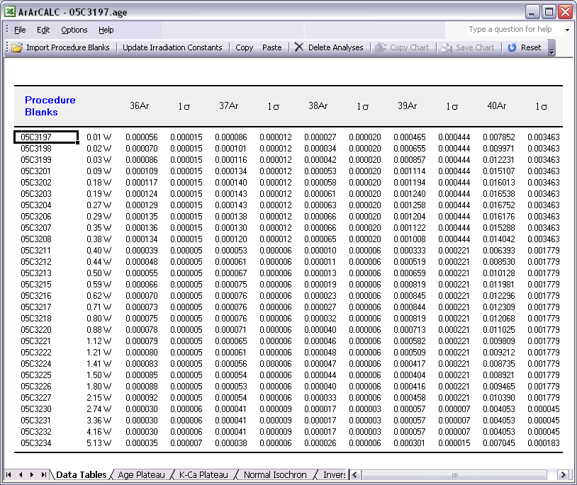
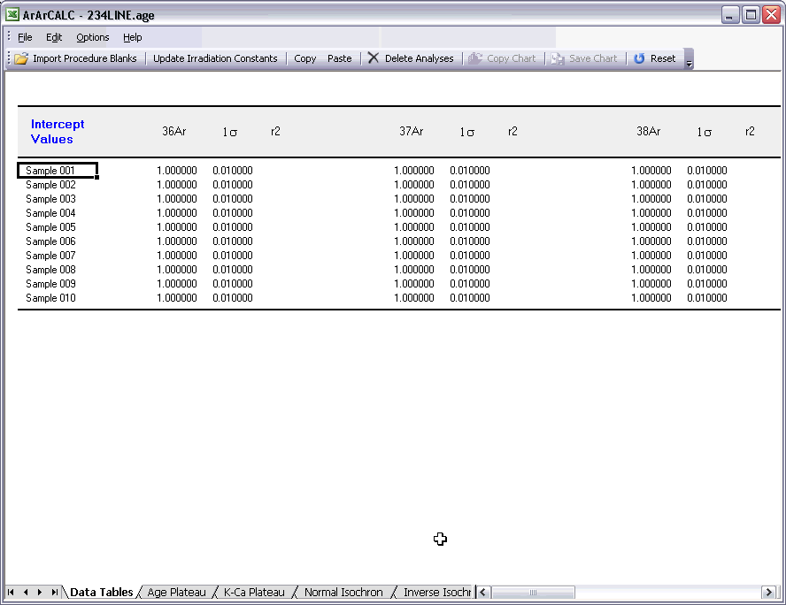
You can edit the intercept values via the Edit # Intercept Values menu item. In this data table all Intercept Values including their 1σ Standard Error (SE) are stored together with the r2, the type of line fit (EXP, PAR, LIN or AVE) and the data points excluded from the data regression. Editing is similar as described above. The Reset button will undo all edits.
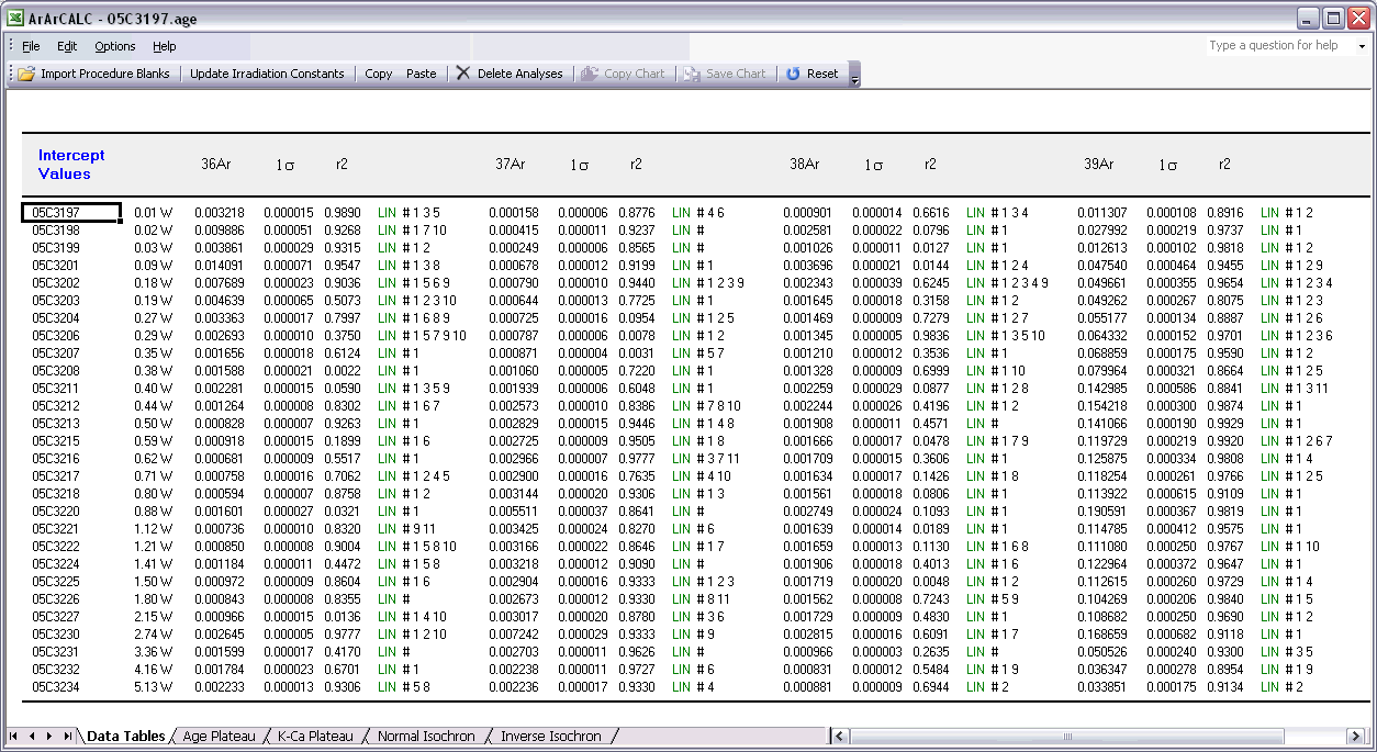
The Sample Parameters (see also: Your First Calculations, Sample Parameters) can be edited via the Edit # Sample Parameters menu. This offers you the possibility to later finalize the actual J-value used in the age calculations or to better define the timing of the measurements. Note that in all the data tables the first two columns on the left (analyses number and increment temperature) cannot be edited. Although there is no possibility (and no need) to edit the analyses numbers, you always can adjust the temperature for each incremental heating step or analysis in the Temp column. All other values can be edited manually. The Reset button will undo all edits.
Finally, the Irradiation Constants may be edited via the Edit # Irradiation Constants menu item. This makes possible the combined age calculation of samples with different irradiation histories (see also: Import Additional Experiments). All irradiation constants can be edited manually. They can also be updated in one go by clicking the Update Irradiation Constants button, which will replace all values with the latest values found in the ArArCALC.log file (see also: Update Irradiation Constants). If you are going to calculate ages in the lunar mode, the labels of this table automatically will be changed from 40/36(a) to 40/36(t) and a default value of 40/36(t) = 1 is assumed (see also: Calculate as Lunar Sample). When you toggle back to the terrestrial age calculation mode, this value gets reset to the default 295.5 value for atmospheric argon. These are the only hard-coded values in ArArCALC and only are applied when toggling to lunar age calculations and back, but you always can overwrite these values by editing the Irradiation Constants table again. The Reset button will undo all edits.

1.5.4 Flagging Analyses in ArArCALC
Of course not every incremental heating experiment is perfectly concordant. So, you need to be able to easily Exclude discordant analyses (or steps) from your (incremental heating) experiments. On this help page three ways to do so are explained.
You can Flag Out your analyses for the age calculations in every data table by double-clicking the Checkmark symbols. When this action is performed ArArCALC recalculates all weighted averages and isochrons automatically, and updates all four diagrams. The total number of analyses included in the calculations are denoted in the Results panel (in this example, n = 14) as well as the total amount of released 39Ar(k) they represent (x = 60.65%). Flagging out multiple analyses is done by right-clicking every analyses that you want to exclude, ending by double-clicking the final one. Repeating these actions will include the analyses again. The Reset button recalculates including all data points.
Flagging Out analyses can also be performed by deselecting points in the isochron diagrams. You can simply do this by left-clicking the data points (green squares) in these diagrams, which change into blue squares when excluded. When this action is performed, ArArCALC recalculates all weighted averages and isochrons. ArArCALC will update all diagrams as well. Flagging out multiple analyses is done by right-clicking every data point that you want to exclude, ending with left-clicking the final one. Repeating these actions on the blue squares will include the analyses again. The Reset button recalculates including all data points.
Raw Data Reduction Line Fit Diagrams
When you calculate line fits in the Raw Data Reduction view, you can exclude data points by either clicking the toolbar buttons 1, 2, 3 ... 11 that represent the data points or by left-clicking the single data points (green squares) on the diagram. Excluded data points are denoted by blue squares and suppressed toolbar buttons. Flagging Out multiple data points can be done by right-clicking each data point and ending with a final left-click. Repeating these actions on the blue squares or the suppressed toolbar buttons will include the analyses again. The Reset button recalculates including all data points.
1.5.5 Deleting Analyses from an ArArCALC File
You can delete analyses from the ArArCALC age calculations files at any time. This can be done from within all nine data tables. However, note that these age calculations files always should include at least two analyses. Select one cell or multiple cells (see below) representing the analyses that you want to delete, and select the Delete Analyses button from the toolbar. Before deleting the analyses, ArArCALC will ask you for a confirmation. ArArCALC will recalculate all ages and update all diagrams when the deletion is confirmed.
2 Function by Function
In this chapter all Functions are explained One-By-One. First the General Functions are explained, which are common to every menu (or view) in the ArArCALC program, followed by the functions that are specific to the Raw Data Reduction and Age Calculation views. Some help topics may have been treated in the Using ArArCALC chapter as well, but in this chapter the functions are explained in more detail.
2.1 General Functions
The File, Options and Help menus contain functions that are common to every view in ArArCALC. These functions are amongst the most used in ArArCALC and range from opening files to printing to exiting to setting preferences and to getting help. However, depending whether you are in the Raw Data Reduction or Age Calculation view, there may be important differences in functionality, which will be explained in this section as well.
2.1.1 Open Datafile
There are three options when selecting the File # Open Datafile # Raw Intensity Data menu item. The first option allows you to open a text file containing your Raw Mass Spectrometry Data ready for data regression. The second option allows you to open an already prepared Age Calculation File, whereas the last option allows you to generate an Empty Age Calculation File (or template file) in which you can enter intensity and blank data manually. This latter option, in particular, is helpful if you want to (re)apply age calculations to old data from your laboratory or from the literature.
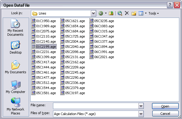
To open a raw intensities data file you should select the File # Open Datafile # Raw Intensity Data (Ctrl+D) menu item. This will give you the following Open DataFile dialogbox. Now browse, select and Open your data file. You can only select one file at a time.
When you have opened your data file, three dialogboxes will be shown to you in sequence. In the first dialogbox, you have to select an Input Filter. In this dialogbox select the input filter that is applicable for the data file you are trying to open. Like in this example, multiple input filters may sometimes be available for different sample types or, if over time, you needed to adjust your input filter(s) because the structure of your data files changed (see also: Setting the Preferences).
In the second dialogbox, you have to set the Sample Type and give an Experiment Name. You always have to make a selection in this dialogbox, but you can always change your settings later, when your data file has been opened successfully in the Raw Data Reduction view (see also: Sample Type and Experiment Name). When filling in the Experiment Name make sure to use unique names (see also: File Name Conventions). In the example below, the Experiment Name is based on the name of the first analysis in an incremental heating experiment. If you are processing data for a single incremental heating experiment, a set of single crystal analyses from one sample or a set of irradiation monitors from the same position in an irradiation package, leave the Experiment Name unchanged so that all your data can be collected and saved in one-and-the-same age calculation file.
In the final dialogbox, you have to set all Sample Parameters that are necessary to perform the age calculations (see also: Sample Parameters). The shown fields are always pre-filled with data from the previous calculation, even if these were performed a few days or weeks ago. Completing this dialogbox will be fast, because most entries will be similar and thus don't need changing. Most likely, only the GMT datum and Temperature need editing, unless you start to reduce a totally new experiment. If your raw data files already have header lines containing this information, ArArCALC will automatically transfer this header information into this dialogbox by using your Input Filter (see also: Setting the Preferences). You can always recall this dialogbox at a later stage in the Raw Data Reduction view via the Options # Sample Parameters menu in order to edit the sample parameters.
When you have entered all the Sample Parameters, you will be guided to the Raw Data Reduction view, where you can regress your argon isotope data by using different line fit methods (see also: Your First Calculation).
Age and Flux Monitor Calculation
To open an age calculation file you should select the File # Open Datafile # Age and Flux Monitor Calculation (Ctrl+A) menu item. This will give you the following Open DataFile dialogbox. Now browse, select and Open your data file. You can only select one file at a time. To open multiple files together, see the Import Additional Experiment help page for more details.
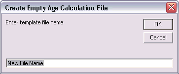
To open an empty age calculation file to use as a template, you should select the File # Open Datafile # Empty Age Calculation File menu item. This is a helpful function that allows you to apply age calculations to old data from your laboratory or from the literature, even if you don't have the original raw data reduction files at hand. Instead you can fill in the regressed intensities of the analyses and, if these are not already blank corrected, you can fill in procedure blanks as well. You first will be asked to give a name for the Empty Age Calculation File.
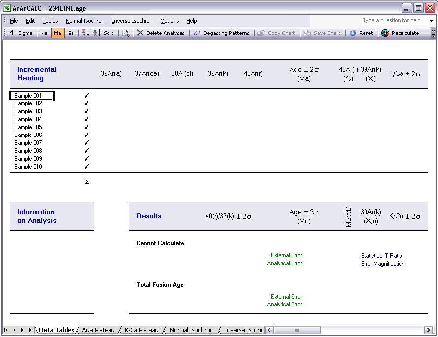
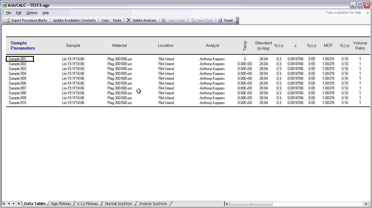
Next an adopted version of the Sample Parameters dialogbox appears, in which you can predefine the number of analyses (or steps) for the experiment. Adjust the spinner button to change the Step Number in the top right panel. In the example below, an Empty Age Calculation File with 10 incremental heating steps is being created. All other fields are similar to the normal Sample Parameters dialogbox and you should fill these out in a similar fashion (see also: Sample Parameters). However, be aware that in this case the dialogbox only appears ones for a single experiment. This means that you should select a Date in the GMT Datum panel that corresponds to the first analysis (or step) in your experiment. Later on you should edit the Sample Parameters table to enter the correct Time values for the incremental heating steps (see also: Editing the Sample Parameters Table). In some cases, you also should edit the Date values, if an experiment runs passed midnight on an experiment day or if a single experiment has be run on separate days. All other parameters always concern the entire experiment, so no extra editing is required.
![]()
When you have clicked the OK button, an Empty Age Calculation File is generated by ArArCALC. As you can see 10 place holders for Sample 001 to 010 have been created, but no calculation is possible since the key input data have not been entered yet (see further below).
Now select the Edit menu in order to start adding (or editing) your data (see also: Edit Menu). In the Intercepts Values table you should replace the 1.000000 and 0.010000 values for the Intensities and Uncertainties of all argon isotopes, respectively. Note that the Uncertainties in this table are always Standard Errors on the 1σ Level. The r2 values are optional.
If the Intercepts Values you entered above are not blank-corrected, you should replace the 0.000000 values for both the Blank Intensities and Uncertainties for all argon isotopes (see below). If the Intercepts Values are already corrected, you can leave the zero blank values in this table. However, in the latter case you should make certain that you have the Apply Procedure Blanks Corrections checkbox unchecked in your Preferences (see also: Preferences), which is the default ArArCALC setting when you generate these template files. Note that the Uncertainties in this table are again Standard Errors on the 1σ Level.
Finally, you should edit the Sample Parameters table. In this table you should (but it is not required) replace the Default Sample Names in the left-most column, the Temp values and you should edit the Date and Time values (not shown below).
When you are finished updating the tables in the Editing view, you should choose the File # Save, Close and Recalculate (Ctrl+S) menu item. Now ArArCALC will check if you have filled in your data correctly and warns you if it encounters problems with your data entries. Otherwise, it will switch back to the Age Calculation view and (re)calculate the ages and plots.
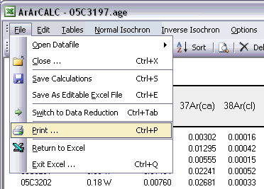
2.1.2 Print
Every data table and diagram is printable from ArArCALC. First select the data table you want to Print via the Table/Edit menu, or select a plateau or isochron diagram using Excel's Worksheet Tabs. Then choose the File # Print (Ctrl+P) menu option.
Check Current Page and select your Paper Size. Then click the Print button and your table or diagram is printed.
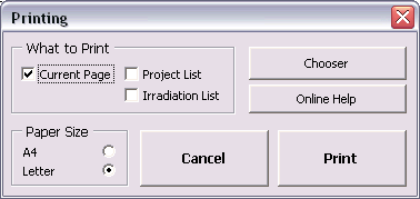
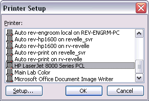
You can select another printer via the Chooser button (see above). This allows you to print in black & white, in color or on transparencies. Click the Setup button (see below) to adjust the settings for the selected printer. These settings will be remembered in between print sessions.
You can further customize your printouts by filling in the Laboratory Identifiers in the Preferences dialogbox (see also: Preferences). These identifiers will always be printed as header and footer, next to the date, time and ArArCALC version number on your printouts. Defining these identifiers is highly recommended, because it will make the archiving of your results more meaningful in the long term.
2.1.5 Irradiations and Projects
ArArCALC saves all age calculation data files in separate directories according to project name (see also: File Organization). This guarantees an automated and well-structured file organization. However, these project names are logged together with all irradiation parameters in the ArArCALC.log file (see also: Using the ArArCALC.log File). This log file can be accessed and updated through a set of easy-to-use dialogboxes. To activate the Changing Irradiations and Projects dialogbox, select the Options # Irradiation and Projects menu item.
The Changing Irradiations and Projects dialogbox lets you choose what via the option buttons Irradiations and Projects in the lower left Change panel. After making a selection, you can use the Add, Edit and Delete buttons to update either the list of project names or irradiations. To add a new list item, you first need to fill in the name of a new irradiation or project in the textbox in the upper right corner, followed by clicking the Add button. To edit or delete an existing irradiation or project, you first click on its name in the list box, followed by clicking either the Edit or Delete button.
If you want to save your edits, please hit the Save button first, because the Close button will close the Changing Irradiations and Projects dialogbox without saving. If you want to ignore or undo any of your changes, hit the Close button without hitting the Save button first.
When adding or editing irradiation definitions, ArArCALC will show you the Change Irradiation dialogbox to allow you to define the irradiation parameters, including up to 999 irradiation segments or cycli (see further below).
information
In this tab you can find summary info and notes for a particular irradiation. In here only the Notes can be edited and it is highly recommended that you provide a short description of the irradiation in this field. This description may include which reactor was
used, whether the samples were shielded or not, the purpose of the irradiation, the related project(s) and what time zone was used in the definition of
the Irradiation Cycli or Segments (see below). The Date and Total Duration of the irradiation are automatically calculated from the Irradiation Cycli
data, where the Date represents the first segment listed in the irradiation list and the Total Duration the summed durations as listed in the first column.
Interference Correction
In this tab you should define the Interference Correction factors and their uncertainties. These constants differ per reactor and whether the samples were shielded or not.
Irradiation segments
In the final tab you can define the Duration, Date, End Time and MW (reactor power) of all Irradiation Cycli or Segments.
It is highly recommended that you use either GMT or your Local Time Zone, as long
as you consistently apply it throughout ArArCALC. For example, you should make certain that you apply the same Time Zone when you define your irradiations and when you supply dates and times in the
Sample Parameters
(see also: Sample Parameters). Use the spin button to increase or decrease the Number of Irradiation Segments. Click on a line in the list box to adjust your settings, which will appear for editing in the
text boxes at the bottom of this dialogbox. To speed up data entry you can also check the Auto Fill option.
2.1.6 Preferences
The program ArArCALC does not contain any constant in its computer code. Every constant, parameter and setting can be set by the user. This is done to give you 100% control over what you calculate in ArArCALC. Below follows a list of adjustable settings in the Preferences dialogbox.
Isochron Settings
These options let you influence the precision of the YORK2 Isochron calculations (see reference: York, 1969). The Convergence determines how small the difference in slope of the isochron should be for two consecutive iterations to result in a successful least-squared fit. The
Convergence is here expressed as a percentage of the slope itself (see also: Isochron Calculations). The number of Iterations determines after how many iterations the isochron calculation should
be terminated, in case the calculation is not converging. If you set the Convergence to a higher precision (a lower percentage),
you also should adjust the number of Iterations accordingly (to a higher number). Clicking the option button Weighted YORK-2 forces ArArCALC to calculate a least-squared linear fit with correlated errors that is weighted by the inverse of the variance (see
reference: York, 1969). You can overrule this setting when performing isochron calculations by selecting
Normal Isochron # Weighted YORK-2
or Normal Isochron # Unweighted YORK-2 in the menu bar.
You can do the same for the Inverse Isochron independently.
Data Reduction Settings
The data reduction settings determine the precision when you apply the Exponential
Fit to your mass spectrometry data. The Convergence is expressed as a percentage of the curvature coefficient that is iteratively derived in this least-squared fit (see also: Line Fitting).
Error Propagation
By checking Irradiation Constants in the Error Propagation box, the errors on the
irradiation correction factors will be propagated in the reported analytical error (see also: Analytical, Internal and External Errors). You can set these errors in the Change Irradiation dialogbox (see also:
Managing Irradiations and Projects). If the Multiply Errors by Sqr(MSWD) is checked, then the errors on the ages and some isotope ratios (e.g. 40Ar/36Ar and 40Ar/39Ar)
will be multiplied by the sqr(MSWD) in case the MSWD becomes larger than 1 (see also: Analytical, Internal and External Errors). Both options are activated by default in ArArCALC.
Ar40, Ar39, Ar38, Ar37 and Ar36
You can chance the option buttons to the right of the Preferences dialogbox in order to set your Default Calculation Type for the raw data reductions
(see also: Line Fitting). You can do this independently for each isotope by choosing from four calculation types: exponentional (Exp), parabolic or second order
polynomial (Par), linear (Lin) and averaging (Ave). You can always overrule these default settings in ArArCALC when performing the actual line
fits.
Other Calculation Settings
With
these checkboxes you can determine which Additional Corrections to apply (or not apply) during the age calculations (see also: Other Calculation Settings). However, it is always recommended that you apply
the corrections for 37Ar and
39Ar Decay following sample irradiation, for
36Ar Ingrowth in chlorine-rich samples, and for Procedure Blanks.
However, for samples younger than 1 Ma it is recommended that you uncheck the Force Negative Intensities to be Zero
... option. This will allow for more accurate age calculations, because
negative ages (or error bars) are statistically expected and valid for these
kind of samples. ArArCALC will generate a
warning when you select a non-default setting.
Defining your own Input Filter is most critical while using ArArCALC. Although it may look complicated, it gives you the flexibility to read-in different types of mass spectrometry data files. ArArCALC does not read-in binary files and expects that the measurements were saved in sequentional text files. Furthermore, the actual intensity measurements should be given per line, including the intensity (in volts, amps or counts) and the time (in hours, minutes or seconds) after inlet of the argon gas in the mass spectrometer. By clicking on the Settings button you can define the internal structure of both the header and data sections in a separate dialogbox (see explanation below). By checking the Choose Input Filter when ... checkbox, ArArCALC allows for the selection of an input filter every time you open a new data file. Otherwise the input filter selected in the list box shown below will be used by default.
General Settings
The File Structure is determined by the Number of Header Rows and the Number of Peak Measurements for each measurement cycle, and whether the
text file is Space, Comma or Tab delimited. The Number of Peaks should be at least five to cover all five argon peaks between Ar36
and Ar40. In the Peak Cycle Structure the user defines which lines represent
peak measurements for the argon isotopes and which lines represent baseline measurements. These lines can be assigned in random order as long as the Number of Peaks is not exceeded.
If you provide two baseline measurements, ArArCALC calculates an average baseline (see Ar36 through Ar39 below). If you provide one baseline measurement, the baseline value will be
subtracted as is (see Ar40 below). You can also fill in "0" when your data already have been baseline corrected (by your data acquisition software, for example). Two positions for the masses
Ar41 and Ar35
have already been reserved for future importing and monitoring of this data.
Record Settings
In the
Record Settings tab you can define which records in the peak lines represent the Peak Measurement, the Error on Peak Measurement and the Time Measurement.
Here you can also define in which units the Time
and Intensity Measurements are given and you can define settings such as
the File Extension, the Maximum Number of Records and Header Lines, and how the Date and Time parameters
and the Errors are represented in the
data files. By default
ArArCALC assumes absolute errors.
Header Structure
Your raw data files may contain more than 1 header line. In the
Header Structure
tab you can define on which header line (H#) and on which record position (R#) the Sample Name or J-Value was stored. This of
course requires that these headers were originally saved in the data file. In the rather simple example below, only one parameter is stored, namely the Number of Cycli, which is stored in the first record of the first header line. Further below a more
complicated example is shown and explained as well.
Example 1 Space delimited text file 1 header line; 10 peak measurements | |
10 5.76734625000000E-0000 9.06800000000003E+0001 3.50166666666667E-0003 1.01855000000000E+0002 1.61403125000000E-0001 1.18145000000000E+0002 3.44500000000000E-0003 1.33135000000000E+0002 6.75000000000000E-0003 1.43025000000000E+0002 3.48000000000000E-0003 1.52855000000000E+0002 3.16950000000000E-0002 1.62740000000002E+0002 3.45666666666667E-0003 1.73865000000002E+0002 1.01312500000000E-0002 1.90145000000000E+0002 3.39500000000000E-0003 2.06435000000001E+0002 5.64673875000000E-0000 2.17610000000001E+0002 3.51833333333333E-0003 2.28845000000001E+0002 1.60882500000000E-0001 2.45105000000000E+0002 3.44000000000000E-0003 2.60125000000000E+0002 6.74500000000000E-0003 2.70010000000000E+0002 3.56250000000000E-0003 2.79840000000000E+0002 etc. etc. |
The number of cycles Cycle 01; Line 01 = mass 40.0; time in seconds Cycle 01; Line 02 = mass 39.5; time in seconds Cycle 01; Line 03 = mass 39.0; time in seconds Cycle 01; Line 04 = mass 38.5; time in seconds Cycle 01; Line 05 = mass 38.0; time in seconds Cycle 01; Line 06 = mass 37.5; time in seconds Cycle 01; Line 07 = mass 37.0; time in seconds Cycle 01; Line 08 = mass 36.5; time in seconds Cycle 01; Line 09 = mass 36.0; time in seconds Cycle 01; Line 10 = mass 35.5; time in seconds Cycle 02; Line 01 = mass 40.0; time in seconds Cycle 02; Line 02 = mass 39.5; time in seconds Cycle 02; Line 03 = mass 39.0; time in seconds Cycle 02; Line 04 = mass 38.5; time in seconds Cycle 02; Line 05 = mass 38.0; time in seconds Cycle 02; Line 06 = mass 37.5; time in seconds etc. etc. |
This is one of the most simple text files possible (see settings in the dialogboxes displayed above). Its space delimited and it has the minimum amount of headers. The Number of Headers should be set to 1 and consequently the Cycle # should be set to [1,1] as well. Since there is only one header line with only one parameter in it, all other possible header positions should be set to zeros (which is the default value). In this example, each measurement cycle produces 10 individual peak measurements (5 isotopic peaks and 5 baselines) and thus the Number of Peaks should be set at 10. The net peak of Ar40 is calculated based on peak 1 minus the average baseline calculated from peak 2 and peak 2, the net peak of Ar39 is calculated based on peak 3 minus the average baseline calculated from peak 2 and peak 4, etc. etc.
Example 2 Comma delimited text file 10 header lines; 6 peak measurements | |
98Haw001 Plagioclase Deep Canyon Anthony Koppers 1100 0.000345,0.3 1.00038,5.7 VU13 12 19-Mar-1999,14:34:03 5.76734625000000E-0000,9.06800000000003E+0001 1.61403125000000E-0001,1.18145000000000E+0002 6.75000000000000E-0003,1.43025000000000E+0002 3.16950000000000E-0002,1.62740000000002E+0002 1.01312500000000E-0002,1.90145000000000E+0002 3.39500000000000E-0003,2.06435000000001E+0002 5.64673875000000E-0000,2.17610000000001E+0002 1.60882500000000E-0001,2.45105000000000E+0002 6.74500000000000E-0003,2.70010000000000E+0002 etc. etc. |
Sample Name Material Location Analyst Temperature J-value and %SD Fractionation correction factor and %SD Irradiation Name The number of cycles Measurement date and time Cycle 01; Line 01 = mass 40.0; time in seconds Cycle 01; Line 02 = mass 39.0; time in seconds Cycle 01; Line 03 = mass 38.0; time in seconds Cycle 01; Line 04 = mass 37.0; time in seconds Cycle 01; Line 05 = mass 36.0; time in seconds Cycle 01; Line 06 = mass 35.5; time in seconds Cycle 02; Line 01 = mass 40.0; time in seconds Cycle 02; Line 02 = mass 39.0; time in seconds Cycle 02; Line 03 = mass 38.0; time in seconds etc. etc. |
This is a more complicated text file that can be read-in by ArArCALC (see settings in the dialogboxes displayed below). Its comma delimited. It has 10 header lines as is set for the Number of Headers. Each measurement cycle produces 6 individual peak measurements (5 isotopic peaks and 1 baseline at mass 35.5), explaining why the Number of Peaks is only set to 6. The net peak of Ar40 is calculated based on peak 1 minus the average baseline calculated from peak 6 and peak 6 (which is the actual baseline value as measured on mass 35.5), the net peak of Ar39 is calculated based on peak 3 minus the average baseline calculated from peak 6 and peak 6, etc. etc.
The number of cycles can be found on the first record of the 9th header line in this text file and the Cycle # is thus set to [9,1]. The Sample Name, Material, Location and Analyst are all located on the first record of header lines 1 through 4. The Temperature for the measurement is located on header line 5, the J-value and Fractionation Correction Factors and their errors are located on header lines 6 and 7 at records 1 and 2, respectively. The Irradiation Name is located on the first record of header line 8. Finally, the Date and Time are located on header line 10 at records 1 and 2 as well. Since the One String for the Data and Time checkboxes have been selected (see above) only one option is available to you for the Date and Time. If you have them unchecked, you can point to individual values for the Day, Month, Year, Hours and Minutes in the header structure.
The Decay Constants and their percentual standard deviations can be set and changed in the Preferences dialogbox below. Here you can also define the data for Decay Activities and Other Physical Constants that are needed for the primary age calculations and recalibrations based on the formulations of Karner & Renne (1998), Renne et al. (1998) and Min et al. (2000). For more details read the Primary Age Recalibration Toolbox help page. The expected units are given in the brackets, unless the numbers are dimensionless.
The information you fill out in the Laboratory Identifiers panel will always be printed as headers and footers, next to the date, time and the ArArCALC version number, when you are making a printout from within ArArCALC. You can also set the File Location of the mass spectrometry data files on your hard disk to ensure that ArArCALC swiftly finds your data files. Finally, you may want to set a Password to protect your settings in the Preferences and Irradiation and Project dialogboxes. Setting passwords is, in particular, advised for the person who is managing the Master ArArCALC.log file, in order to circumvent accidental deletion of these important parameters (see also: Using the ArArCALC.log File).
2.1.8 ArArCALC Online Help
This ArArCALC package comes with help files written in HTML that are accessible through your web browser. These help files can be reached when running ArArCALC through the Help menu by selecting the ArArCALC Online Help (Ctrl+H) menu item. Note that these help files are not locally stored on your hard drive. This setup allows you to retrieve the most up-to-date help files without downloading the updated help files to your own computer. The ArArCALC Help Library will be launched in your default browser with the Table of Contents as the first page.
Most dialogboxes used in ArArCALC also have Online Help buttons. Click on these buttons to retrieve "context sensitive help" information from the help files stored in this online ArArCALC Help Library.
2.1.9 ArArCALC on the Web
The ArArCALC Website is continuously maintained at http://earthref.org/tools/ararcalc.htm. You can reach this website by placing a bookmark in your web browser, but you can also select the ArArCALC on the Web (Ctrl+W) menu item from within the ArArCALC software itself. On the ArArCALC Home Page you will find links to the latest downloads and news on the ArArCALC program. The website will be launched in your default browser.
2.1.10 About ArArCALC
If you want to verify what version of ArArCALC you are currently using, select the Help # About ArArCALC menu item. A window will appear (and disappear after a few seconds) that is the same as the splash window shown during the startup of ArArCALC. This window contains the basic information about the ArArCALC software and its developer.
2.2 Raw Data Reduction
Functions that are specific to the Raw Data Reduction view will be discussed in this section. Some can be found in the File and Options menus and allow you to save your data regressions and change your sample parameters. However, the most important and most frequently-used functions you will find on the ArArCALC Toolbar. From this toolbar you can toggle data points in the data regressions, select different type of regressions, swap between the Ar36, Ar37 ... Ar40 argon isotopes, and more.
2.2.1 Save
ArArCALC saves all calculated argon intensities of a single experiment in a single Microsoft Excel Workbook that includes two plateau diagrams, two isochrons, and their respective data tables. To save your calculated Ar40, Ar39 ... Ar36 intensities, choose File # Save (Ctrl+S) from the menu bar. ArArCALC first checks if you have performed calculations for all five argon isotopes. If not, it will warn you that your calculations cannot be saved at the moment. Otherwise, it saves your calculations in the Age Calculation File that is stored in the user-defined Project directory with a file name based on the given Experiment Name. However, if you have been performing data reductions for Blank or Air data, your calculations will be saved in Text Files instead. These files are by default stored in the ArArCALC/Blanks and ArArCALC/Airs directories, based on the Measurement Date and the Experiment Name, respectively.
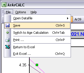
2.2.2 Switch to Age Calculation
Switching from the Raw Data Reduction view to the Age Calculation view while saving your calculations is very simple. To do so, you should select the File # Switch to Age Calculation (Ctrl+Tab) menu option. Your calculations will be automatically saved (see also: Saving Data Reductions) and, if not possible, you will be notified with a warning. This functionality allows you to reduce your argon mass spectrometry data and then directly switch to the age calculations to check on the results. During this switching you can always suppress the saving, if you hold down the SHIFT key.
2.2.3 Sample Parameters
As an ArArCALC user you have to set the Sample Parameters every time you open a Raw Mass Spectrometry data file (see also: Open Datafile). While you are performing the data regressions for these data, you can always recall this dialogbox via the Options # Sample Parameters menu in order to adjust your settings. The shown fields are always pre-filled with data from the previous calculation, even if these were performed a few days or weeks ago. Completing this dialogbox will be fast, because most entries will be similar and thus don't need changing when regression data from a single (incremental heating) experiment. Most likely, only the GMT datum and Temperature need editing, unless you start to reduce a totally new experiment. If your raw data files already have header lines containing this information, ArArCALC will transfer this header information into this dialogbox by using your Input Filter (see also: Setting the Preferences).
Information Panel
It is recommended that you use (as) descriptive (as possible) entries in the Information panel. Fill in sample name and position in the irradiation container in the Sample field, fill in mineral, rock type and grain size fraction in the Material
field, and enter full names (instead of initials) in the Analyst
field (see also: How to Insert Symbols in Microsoft Excel). In the Location
field try to fill in the "true" location name or (if not available) the name of the region or country (in order of preference). Finally, in the Temperature field fill in the incremental heating settings in either °C,
laser power in W or laser power in %. Don't enter the units here since you already predefined these in the Input Filter that you used while opening the data file (see also: Preferences).
You can always overwrite these default settings by selecting the correct unit from the Options # Heating Unit menu (see also: Heating Unit) when you are in the Age Calculation
view.
Correction Factors Panel
In this panel you have to fill in some of the most crucial Correction Factors that are required for the age calculations. First of all, you need to fill in the Standard Age (in Ma)
including its proper Standard Name. Next you have to fill in the infamous J-value, the Mass Discrimination Factor (see also: Mass Discrimination Corrections),
any needed Volume Correction (if you split your gas sample in any way) and the Sensitivity (in mol/volt). Because you have to provide both a Standard Age and the J-value,
this allows ArArCALC to calculate the data either as a flux monitor or as an unknown (see also: Calculate as Flux Monitor).
Resistance on Amplifier Panel
These options are only relevant if you have installed a Variable Resistor on the amplifier, which you can (automatically) switch according to the amount of gas introduced into your mass
spectrometer. Select the correct resistance value in order to let ArArCALC normalize the measured intensities to the Default Resistor (109) value. This means that when you select the 108 resistor
value that the intensities reported in ArArCALC are 10x higher than measured, and when you select the 107 value that the intensities reported are 100x higher. If you operate with a fixed resistor, you always should keep the default option selected
(see example above).
Identifiers Panel
This panel contains two list boxes in which you can select the Irradiation for your sample and under which Project to store the age calculations. Both lists
you manage yourself in the Irradiations and Projects dialogboxes and you should make certain that you have entered the appropriate irradiation and project for the sample you are currently processing (see also: Irradiations and Projects).
GMT Datum Panel
You have to set the Inlet Time of the argon gas in the mass spectrometer in this panel. Provide this information as the day (d), month (m), year (y), hour (h) and minute (m) by adjusting the spinner
buttons. Although it is preferred that you enter all times in GMT (Greenwich Mean Time), you can also provide local times in this panel. However, in the latter case, you should also make certain that the irradiation times were provided in the same time zone
units (see also: Irradiations and Projects) and that you take care of daylights saving time (if applicable in your country). It is highly recommended that you Date and Time
Stamp your data files, so that you automatically can read in this information from the header in these files (see also: Configuring the Input Filter).
2.2.4 Sample Type and Experiment Name
Every time you open a Raw Mass Spectrometry data file (see also: Open Datafile) you have to specify the Sample Type and the Experiment Name under which you want to save the data to be used in your age calculations. While you are performing the data regressions for these data, you can always recall this dialogbox via the Options # Sample Type menu.
When filling in the Experiment Name make sure to use unique names (see also: File Name Conventions). In the example below, the Experiment Name is based on the name of the first analysis in an incremental heating experiment. If you are processing data for a single incremental heating experiment, a set of single crystal analyses from one sample or a set of irradiation monitors from the same position in an irradiation package, leave the Experiment Name unchanged so that all your data can be collected and saved in one-and-the-same age calculation file.
2.2.6 Ar40. Ar39 ... Ar36 Buttons
In the Raw Data Reduction view, a XY-scatter plot displays the measurement time (in seconds) after the inlet of the argon sample in the mass spectrometer on the X-axis, and the intensity of the beam on the Y-axis (in volts, amps or counts). By default, the intensity data for Ar40 is shown first (see below). Each different argon isotope should be calculated by clicking the isotope buttons Ar40, Ar39 ... Ar36 before you can save the data regressions.
2.2.7 EXP, PAR, LIN and AVE Buttons
When performing data regressions, ArArCALC does not decide which fit to the data (exponentional, parabolic, linear or average) gives the best results. For this purpose, you can set the default regression type for each argon isotope in the preferences (see also: Calculation Preferences). Only in one particular case, when the exponential and parabolic are similar to the linear least-squared fit, ArArCALC accepts a linear fit by default. However, based on the calculation results (see the boxes to the right of the scatter plot) you can always overrule these program decisions yourself, by choosing the appropriate button on the ArArCALC toolbar: Exp, Par, Lin or Ave. In the example below the parabolic fit has been chosen by the user.
2.2.8 Copy Chart
Click the Copy Chart button on the ArArCALC toolbar to copy the active chart to the Clipboard. Now you can paste the chart into your favorite drawing program, such as Adobe Illustrator, Canvas or CorelDraw. Most importantly, the copied chart will be pasted as Vector Graphics and thus it allows you to edit each drawing object and line in the diagram. However, in order to proceed, you first have to release all the masks, compound paths and/or groups. Do this on the entire selection at once. After these actions, you can always group together the age plateau lines (for example) by first selecting the line segments based on the color and weight of the line and then by selecting the group option. This will make working with these files more easy for you.
2.2.9 Save Chart
Click the Save Chart button on the ArArCALC toolbar to save the active chart as a GIF Image to your hard disk. The file will be saved in the Project Folder by default, that is the same folder as where your age calculation file is being saved. In addition, ArArCALC will name the the GIF Image based on the Experiment Name, alike the age calculation file.
2.2.13 Reset
The Reset button recalculates the data regressions including all data points. However, note that only the data points for the currently selected isotope will be reset.
2.3 Age Calculations
Functions specific to the Age Calculation view will be discussed in this section. Saving, exporting and closing age calculations files all are done from the File menu, while many advanced (calculation) functions are available from the Options menu. You can use the Edit and Table menus to navigate between the nine data tables in which ArArCALC stores your data, and you can use the Normal and Inverse Isochron menus to set your preferences for the isochron calculations and their display options.
2.3.1 Close
Select the File # Close (Ctrl+X) menu item to Close the active age calculation file. In all cases your age calculation file will be saved upon closing (even though no progress bar is shown).
2.3.2 Save Calculations
To Save your calculations select the File # Save Calculations (Ctrl+S) menu item. This also will save your user preferences, calculation settings and irradiation definitions, as they are stored in your age calculation file. During saving the latest ArArCALC Version Number is added to the properties of the file itself, which you can view by selecting the File Properties within Windows Explorer. A progress bar appears, showing you the status while saving.
2.3.3 Export for Publication
The standard Age Calculation workbooks with the extension *.AGE cannot be opened in Microsoft Excel 2000-XP-2003 without running ArArCALC. These files are password protected to circumvent the possibility of (unexpected) changes made to the workbooks, leaving these files unreadable by ArArCALC itself. However, if you save your calculations via the File # Save as Editable Excel File (Ctrl+E) option, the password protection and the Microsoft Excel macros are removed. Now you can open these newly-saved files with the extension *.XLS in Microsoft Excel and change the format of their data tables and diagrams manually. A progress bar appears, showing you the status while saving these editable files.
2.3.5 Switch to Data Reduction
Switching from the Age Calculation view to the Raw Data Reduction view is very simple. To do so, you should select the File # Switch to Data Reduction (Ctrl+Tab) menu option.
2.3.6 Edit Menu
Four data tables in ArArCALC include data necessary for the age calculations, but which you always can edit. These data tables are all located in the Data Tables worksheet and can be selected through the Edit menu. You can also use the F1, F2, F3 and F4 keyboard strokes for faster navigation between these tables.
ArArCALC has been set-up to run on-line during mass spectrometry and by default uses the latest-calculated blank measurement for its blank corrections. However, you can always edit the blank intensities later via the Edit # Procedure Blanks menu item. This function displays a data table containing Blank Intensities and their 1σ Standard Error (SE) for each analysis (step) in your (incremental heating) experiment. You can edit these blank data by clicking the cells and typing in new values. A single click lets you replace the complete number, whereas double-clicking will allow you to edit the number within its cell. To copy values from one cell to another, use the Drag functions of Microsoft Excel (drag the black square anchor visible on the highlighted cell down or to the right) or use the Copy (Ctrl+C) and Paste (Ctrl+P) buttons. Note that you can also copy blank values via the clipboard, in which case you select the cells in which to place your new values and use the Paste (Ctrl+P) button. The Reset button will undo all edits, unless you already have saved them.
You can also select single (or multiple) cells, representing one (or more) analyses, and then choose Import Procedure Blanks from the toolbar. Since ArArCALC saves all blank measurements in text files organized per measurement date, this function allows you to import multiple blank measurements for a range of days, by opening more than one of these text files. Blank measurements can now be selected in the Select Blank Files list box to calculate Average Blanks for all argon isotopes, including their (predicted) standard deviations. This ArArCALC tool then automatically replaces all blank values and uncertainties in the edit table for the selected analyses. However, when the Default Errors checkbox is checked, the standard deviations will be overruled by percentual errors.
![]()
You can also click the Advanced Blanks button to analyze the Evolution in the Procedure Blanks over the same range of days. For each argon isotope you can now calculate a linear, parabolic or polynomial fit (pink dashed line). These calculations can be done while generating a standard error or 65-95% confidence envelop (grey dashed lines). The unknowns for which to calculate the blank values are indicated by gray circles at the bottom of the diagram (see also: Import Procedure Blank Toolbox). When you click the OK button, this ArArCALC tool again replaces all blank values and uncertainties in the edit table for the selected analyses.
![]()
You can edit the intercept values via the Edit # Intercept Values menu item. In this data table all Intercept Values including their 1σ Standard Error (SE) are stored together with the r2, the type of line fit (EXP, PAR, LIN or AVE) and the data points excluded from the data regression. Editing is similar as described above. The Reset button will undo all edits.
The Sample Parameters (see also: Your First Calculations, Sample Parameters) can be edited via the Edit # Sample Parameters menu. This offers you the possibility to later finalize the actual J-value used in the age calculations or to better define the timing of the measurements. Note that in all the data tables the first two columns on the left (analyses number and increment temperature) cannot be edited. Although there is no possibility (and no need) to edit the analyses numbers, you always can adjust the temperature for each incremental heating step or analysis in the Temp column. All other values can be edited manually. The Reset button will undo all edits.
Finally, the Irradiation Constants may be edited via the Edit # Irradiation Constants menu item. This makes possible the combined age calculation of samples with different irradiation histories (see also: Import Additional Experiments). All irradiation constants can be edited manually. They can also be updated in one go by clicking the Update Irradiation Constants button, which will replace all values with the latest values found in the ArArCALC.log file (see also: Update Irradiation Constants). If you are going to calculate ages in the lunar mode, the labels of this table automatically will be changed from 40/36(a) to 40/36(t) and a default value of 40/36(t) = 1 is assumed (see also: Calculate as Lunar Sample). When you toggle back to the terrestrial age calculation mode, this value gets reset to the default 295.5 value for atmospheric argon. These are the only hard-coded values in ArArCALC and only are applied when toggling to lunar age calculations and back, but you always can overwrite these values by editing the Irradiation Constants table again. The Reset button will undo all edits.
2.3.7 Tables Menu
Nine different data tables are available in every ArArCALC age calculation file. Five of these tables include output data from your age calculations, whereas four tables include the input data necessary to perform the age calculations and which you can edit at any time (see also: Editing Data in ArArCALC). The calculation data tables are all located in the Data Tables worksheet and are selectable through the Tables menu. You can also use the F5, F6, F7, F8 and F9 keyboard strokes for faster navigation between the tables.
The Age Plateau data table contains calculation data for the plateau age, total fusion ages and K/Ca ratios. Note that also the MSWD, the number of increments and the total amount of 39Ar(k) in percent are given for the age plateau calculation. The uncertainties on the 40Ar/39Ar ages are defined as Internal Errors that combine the Analytical Errors with the Errors on the J-value. For completeness, the Analytical Errors and External Errors (including the error on the total 40Ar decay constant) are given as well (see also: Analytical, Internal and External Errors). The checkmarks signify the analyses included in the age plateau calculation, whereas the summed 36Ar(a), 37Ar(ca), 38Ar(cl), 39Ar(k) and 40Ar(r) components at the bottom of the table are used to calculate the total fusion (or recombined) age.
The Normal Isochron and Inverse Isochron data tables contain the calculated ratios 39Ar/36Ar, 40Ar/36Ar, 39Ar/40Ar and 36Ar/40Ar as used in the York (1969) isochron calculations. Both tables display correlation coefficients (r.i) denoting to what extend the errors used in these isotope ratios are correlated. In the example of an inverse isochron below, the correlation is minimal, because the error in the 40Ar (denominator) is small compared to the errors on 39Ar and 36Ar (the nominators). In the Statistics section the isochron calculations are further described by the convergence, number of iterations, type of calculated line, F-ratio, error magnification factor, and the number of points included in these calculations.
The Degassing Patterns data table contains for every analyses in your experiments the calculated argon components. For example, the entire measurement for the 36Ar isotope can be divided into the 36Ar(a) atmospheric, 36Ar(ca) calcium and 36Ar(cl) chlorine components, and if you are analyzing lunar rocks, also the 36Ar(c) cosmogenic component. For each individual component all increments or steps are summed, while the components themselves are summed as well (see the bottom of the table). A selection of these summed components appears in the Age Plateau data table as well (see above) and they are used to calculate the total fusion ages or to display these in the isochron diagrams (see also: Total Fusion Points in Isochron Diagrams). You can also visualize the Degassing Patterns in an interactive toolbox (see also: Degassing Patterns Toolbox).
The last data table for Additional Parameters contains an extra selection of data that may be interesting to you when judging the outcome of your argon experiments. Most notable are the decay correction factors for 37Ar and 39Ar, which are used to correct for radioactive decay occurring between the irradiation of the sample and your actual measurements. But also the absolute amount of 40Ar measured is listed here in moles, and the corrected 40Ar/39Ar, 37Ar/39Ar and 36Ar/39Ar ratios and their uncertainties.
2.3.8 Normal and Inverse Isochron Menus
Individual menus are available for the Normal and Inverse Isochrons, allowing you to change a variety of Display options for each isochron separately and to toggle the calculations between Weighted/Unweighted YORK-2 Fits.
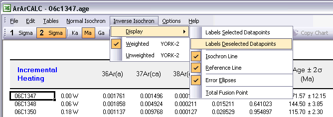
Display Labels for Selected Data Points
You can show or hide Labels for the Selected data points (green squares) in your isochron diagrams by toggling this menu item. The labels always show you the Temperature for a specific (incremental heating) data point. For example, 0.06W or 1500°C.
Display Labels for Deselected Data Points
Alternatively, you can show or hide the same Temperature Labels for the Deselected data points (blue squares).
With this menu item you can show or hide the calculated Isochron line (pink line). The isochron line is shown by default, except if less than 3 data points are included in the calculations.
You can also show or hide the Reference line (dark grey line) that depicts the line between the Plateau Age Intercept on the 39Ar/40Ar axis and the Atmospheric Argon Intercept (295.5) on the 36Ar/40Ar axis. In a perfect case, the reference and isochron lines overlap on the 95% confidence level. The reference line is shown by default, except if less than 3 data points are included in the calculations.
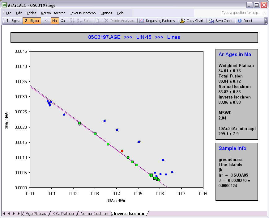
To show or hide Error Ellipses in the isochron plots toggle this menu item. Since the ratios on the axes of the isochron diagrams have errors that are correlated, the ellipses always become (slightly) inclined. This is more clear in normal isochrons than in inverse isochrons, where in the normal isochron diagrams the ellipses often get elongated extensively and rotated to line up with the isochron itself. In that case, it is often easier to hide the error ellipses from view, which also is the default setting in ArArCALC for normal isochrons. For the inverse isochrons, the ellipses are shown by default.
The Total Fusion Point (red circle) can be shown or hidden in both isochrons. By default ArArCALC shows this point, because in a closed system, this point is expected to coincide with (i.e. falling on) the isochron line. These points thus provide you with an easy visual check on this particular characteristic for your sample.
By default the Isochron calculations are performed using Weighted Errors (York, 1969).
In some cases, you might want to use an Unweighted YORK-2 Fit. A good example is, if one of your data points has an unusual small error (because you employed a too large incremental heating step) and thus (unrealistically) outweighs all other data points in your isochron calculations. By choosing this option, a linear fit without any weighting gets performed, and thus ignores the unevenness in your heating schedule.
2.3.9 Heating Unit
You can set the Heating Unit for your sample to either Laser Wattage, Laser % or Temperature (in °C). Simple select your option from the Options # Heating Unit menu item, and the tables in ArArCALC will automatically be updated and reformatted.
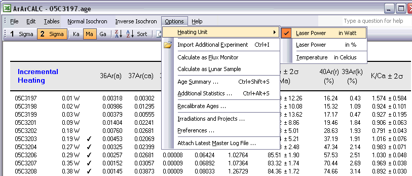
2.3.10 Import Additional Experiment
You can also Combine Multiple Experiments in single ArArCALC age calculation workbooks, when using the Options # Import Additional Experiment menu item. This functionality allows you to combine analyses from co-magmatic mineral separates (e.g. plagioclase and hornblende) from one rock sample into a single isochron calculation. Also, multiple total fusion experiments for one flux monitor standard can be merged into one calculation. Finally, this functionality allows you to combine or directly compare sample splits measured in different laboratories or from different irradiations.
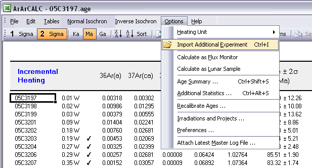
2.3.11 Calculate as Flux Monitor
Choosing the Options # Calculate as Flux Monitor menu item toggles between calculation of J-values and ages. This is possible since ArArCALC requires the input of both the standard age and J-value (and their uncertainties) for every analysis (see also: Your First Calculation ... How to Start). This functionality may be useful to you, when you are reducing data from flux monitor standards, for which both the resulting standard age and J-value are of interest.
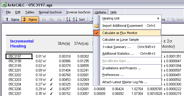
2.3.12 Calculate as Lunar Sample
Choosing the Options # Calculate as Lunar Sample menu item toggles between calculation of terrestrial and lunar ages. When calculating Lunar Ages the atmospheric component is replaced with a trapped component and an additional cosmogenic component is added into your calculations.
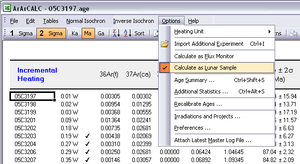
2.3.14 Display Additional Statistics
Choosing the Options # Additional Statistics menu item displays a dialogbox containing a summary of the plateau age (or J-value), plus a list of additional statistical parameters describing the shape and form of the plateau itself. The perfect (flat) age plateau would have a slope and skewness of zero, a high positive kurtosis and a low square of deviations.
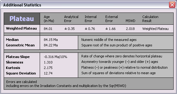
2.3.20 Attach Latest Master Log File
In some cases, you may want to replace the log files that are attached to your age calculation files with the latest Master ArArCALC.log file. Select the Options # Attach Latest Master Log File menu item. First the old log files will be removed from your Excel workbook, where after a copy of the latest master settings will be appended again (see also: Using the ArArCALC.log File). Before replacing the log files, you will be asked to confirm this action.
2.3.22 Ka, Ma and Ga Buttons
You can report your age data either in Ka, Ma or Ga units. Click the appropriate button in the ArArCALC Toolbar and your data will be recalculated and reformatted accordingly. Ma is the default setting in ArArCALC.
![]()
2.3.23 Table Sorting
You can sort the data tables by selecting any cell in the column on which you like to sort and then hit one of the Sort buttons. The sort can be performed in a descending (first button) or ascending (second button) order. You can sort using up to three different sorting keys. To use more than one sorting key, you should select up to three different cells in three different columns while holding down the CTRL button and then hit one of the Sort buttons. To restore the default sorting order, you should sort on the first column, as shown in each table, or on the temperature column in case of an incremental heating experiment.
![]()
2.3.24 Table Zooming
You can Zoom In on the text in the data tables by clicking on the Magnification Glass button in the ArArCALC Toolbar. To restore the view, select the 100% zoom level after clicking the Magnification Glass button again.
![]()
2.3.25 Delete Analyses
You can always delete analyses from your age calculation files. Simply select one or more analyses in the data table and click Delete Analyses on the ArArCALC Toolbar. You will be asked to confirm the deletion.
![]()
2.3.26 Degassing Patterns Toolbox
The degassing of whole rock and basaltic groundmass samples during incremental heating experiments can be rather complex (for example Koppers et al. 2000 and 2004). The Degassing Patterns Toolbox is provided to you to better study and understand these degassing behaviors. In the example below of a submarine groundmass sample, the measured intensities of four argon components are shown, as indicated by the orange, purple, light blue and green buttons in the Select Argon Components panel. This is an interesting view of the degassing behavior of this sample, but the signal is rather erratic and the high intensity for the 40Ar(r) Component forces the other components to be nearly invisible near the bottom axis. This view becomes much more useful, if we normalize the signal (i.e. intensity) to the step size, as shown in the second example below. The 40Ar(r) Component now closely resembles the shape of the age spectra, which is what we are expecting, yet its intensity still overwhelms the other components. This problem gets alleviated as well, if we plot the degassing patterns as fractions over the entire experiment. This is shown in the third example below and clearly brings forward the low intensity components in the same plot. As it turns out, this experiment shows large spikes in the 36Ar(a) and 38Ar(cl) Components for the low temperature increments and another spike in the 37Ar(ca) Component for the high temperature increments. These are very useful observations that will help you in the interpretation of complex argon age spectra.
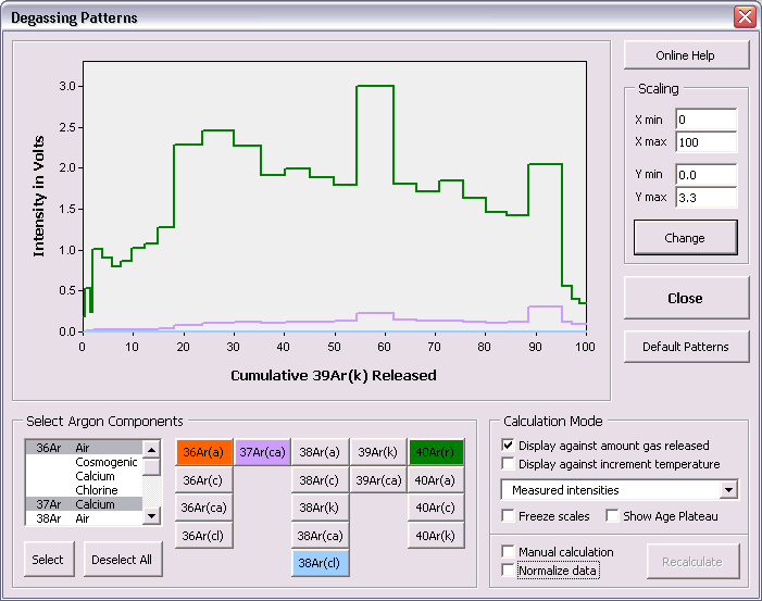
Select Argon Components
To select or deselect certain Argon Components, click either on the buttons or make your selections in the list box on the left-hand side. You can also use the buttons beneath this list box to Select All or
Deselect All. The colors of the selected buttons correspond to the colors of the lines in the diagram.
Calculation Mode
By default the data are plotted against the Cumulative Amount of 39Ar(k) Released. However, you can also display the data against the Increment Temperature in case of a incremental heating experiment.
Select one of the two checkboxes to change between these modes. Freeze Scales is helpful when you want to save the scaling settings between different toolbox sessions. You can also select the Show Age Plateau checkbox, which will
add a horizontal bar to the plot, indicating the position of the age plateau. Check the Normalize Data checkbox if you want the normalize the intensities measured against the step size or the amount of 39Ar(k) in
each increment. And, finally, you can disable the automatic updating of the plot and do a Manual Calculation. In that case use the Recalculate button to update the calculations.
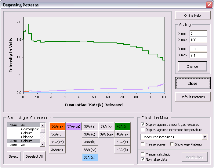
Scaling
To manually scale the plot, change the numbers in the Scaling panel and click on the Change button. If you want to retain these customs settings between different toolbox sessions, be certain to check the Freeze Scale
checkbox.
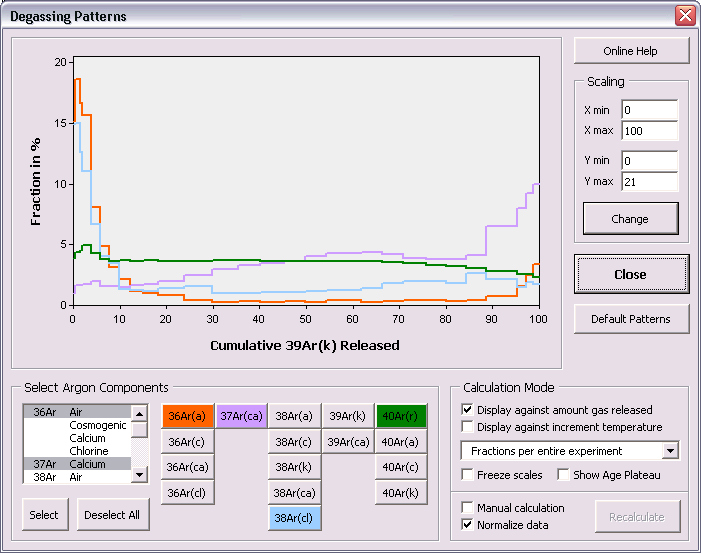
2.3.27 Copy Chart
To use or edit your plateau and isochron diagrams in your favorite drawing program, click the Copy Chart button on the ArArCALC Toolbar. Your diagrams will be put onto the clipboard in a vector graphics format and can be pasted straight into software tools like Adobe Illustrator, Canvas or CorelDraw (see also: Working with ArArCALC Diagrams in Adobe Illustrator).
![]()
2.3.28 Save Chart
You can also save your plateau and isochron diagrams as a GIF Image by clicking the Save Chart button on the ArArCALC Toolbar. The image files will be saved automatically in your Project folders (see also: File Organization).
![]()
2.3.29 Reset
By clicking the Reset button on the ArArCALC Toolbar you will include all "unflagged" analyses in your calculations again. Upon calculation all tables and diagrams will be updated accordingly (see also: Flagging Analyses in ArArCALC).
![]()
2.3.30 Recalculate
Click the Recalculate button on the ArArCALC Toolbar if you want to refresh the age calculations. In most cases, this is not necessary, because ArArCALC automatically recalculates the ages when you make changes. There is one exception, however, that is when you have updated your preferences or irradiation constants (see also: Preferences, Irradiations and Projects). In that case, your new settings will be applied when you hit the Recalculate button or when ArArCALC recalculates because you made other changes to the age calculation file. Examples of the latter are the (un)flagging of your analyses, adding or deleting analyses, changing the 1 or 2 sigma confidence level, changing the age units, etc.
![]()
2.5 Editing Mode
The functions available to you in the Edit Mode will be discussed in this section. Saving, recalculating and closing of your edits is done from the File menu, while you still can use the Edit menu to navigate between the four edit tables. A handful of advanced tools are available from the ArArCALC Toolbar, allowing you to Import Procedure Blanks or to Update Irradiation Constants in an easy fashion.
2.5.1 Save, Close and Recalculate
When you are finished editing your data in one or more of the four edit tables, you should apply these by selecting the Files # Save, Close and Recalculate (Ctrl+S) menu item. A progress bar appears, showing you the status while applying your edits. When all edits have been applied, you will be returned to the Age Calculation mode. If you have entered data in the wrong format, outside their allowed data range, or you have left some of the required fields blank, ArArCALC will ask you to change the particular data field(s) first.
2.5.2 Close Without Saving
If you want to leave the Edit Mode without saving your edits, select the Files # Close Without Saving (Ctrl+X) menu item. You edits will be undone first (see also: Reset) after which you will be returned to the Age Calculation mode.
2.5.3 Edit Menu
Four data tables in ArArCALC include data necessary for the age calculations, but which you always can edit. These data tables are all located in the Data Tables worksheet and can be selected through the Edit menu. You can also use the F1, F2, F3 and F4 keyboard strokes for faster navigation between these tables.
ArArCALC has been set-up to run on-line during mass spectrometry and by default uses the latest-calculated blank measurement for its blank corrections. However, you can always edit the blank intensities later via the Edit # Procedure Blanks menu item. This function displays a data table containing Blank Intensities and their 1σ Standard Error (SE) for each analysis (step) in your (incremental heating) experiment. You can edit these blank data by clicking the cells and typing in new values. A single click lets you replace the complete number, whereas double-clicking will allow you to edit the number within its cell. To copy values from one cell to another, use the Drag functions of Microsoft Excel (drag the black square anchor visible on the highlighted cell down or to the right) or use the Copy (Ctrl+C) and Paste (Ctrl+P) buttons. Note that you can also copy blank values via the clipboard, in which case you select the cells in which to place your new values and use the Paste (Ctrl+P) button. The Reset button will undo all edits, unless you already have saved them.
You can also select single (or multiple) cells, representing one (or more) analyses, and then choose Import Procedure Blanks from the toolbar. Since ArArCALC saves all blank measurements in text files organized per measurement date, this function allows you to import multiple blank measurements for a range of days, by opening more than one of these text files. Blank measurements can now be selected in the Select Blank Files list box to calculate Average Blanks for all argon isotopes, including their (predicted) standard deviations. This ArArCALC tool then automatically replaces all blank values and uncertainties in the edit table for the selected analyses. However, when the Default Errors checkbox is checked, the standard deviations will be overruled by percentual errors.
![]()
You can also click the Advanced Blanks button to analyze the Evolution in the Procedure Blanks over the same range of days. For each argon isotope you can now calculate a linear, parabolic or polynomial fit (pink dashed line). These calculations can be done while generating a standard error or 65-95% confidence envelop (grey dashed lines). The unknowns for which to calculate the blank values are indicated by gray circles at the bottom of the diagram (see also: Import Procedure Blank Toolbox). When you click the OK button, this ArArCALC tool again replaces all blank values and uncertainties in the edit table for the selected analyses.
![]()
You can edit the intercept values via the Edit # Intercept Values menu item. In this data table all Intercept Values including their 1σ Standard Error (SE) are stored together with the r2, the type of line fit (EXP, PAR, LIN or AVE) and the data points excluded from the data regression. Editing is similar as described above. The Reset button will undo all edits.
The Sample Parameters (see also: Your First Calculations, Sample Parameters) can be edited via the Edit # Sample Parameters menu. This offers you the possibility to later finalize the actual J-value used in the age calculations or to better define the timing of the measurements. Note that in all the data tables the first two columns on the left (analyses number and increment temperature) cannot be edited. Although there is no possibility (and no need) to edit the analyses numbers, you always can adjust the temperature for each incremental heating step or analysis in the Temp column. All other values can be edited manually. The Reset button will undo all edits.
Finally, the Irradiation Constants may be edited via the Edit # Irradiation Constants menu item. This makes possible the combined age calculation of samples with different irradiation histories (see also: Import Additional Experiments). All irradiation constants can be edited manually. They can also be updated in one go by clicking the Update Irradiation Constants button, which will replace all values with the latest values found in the ArArCALC.log file (see also: Update Irradiation Constants). If you are going to calculate ages in the lunar mode, the labels of this table automatically will be changed from 40/36(a) to 40/36(t) and a default value of 40/36(t) = 1 is assumed (see also: Calculate as Lunar Sample). When you toggle back to the terrestrial age calculation mode, this value gets reset to the default 295.5 value for atmospheric argon. These are the only hard-coded values in ArArCALC and only are applied when toggling to lunar age calculations and back, but you always can overwrite these values by editing the Irradiation Constants table again. The Reset button will undo all edits.
2.5.4 Import Procedure Blank Toolbox
This special toolbox is provided to help you analyze the Evolution of your Procedure Blanks over a single day or a range of days. To use this toolbox, first activate the blanks table via the Edit # Procedure Blanks menu item. Now select one or more analyses and click the Import Procedure Blanks button on the ArArCALC Toolbar. Since the blank measurements are all saved in text files organized by measurement date, this tool allows you to import multiple blank measurements for a range of days, by opening more than one of these text files. Hold down the control key when selecting more than one file.
![]()
The Advanced Blank Calculations dialogbox is now shown, in which you can select/deselect blanks and go through the Ar36, Ar37 ... Ar40 isotopes to calculate either a Linear, Parabolic, Polynomial or Average Fit (pink dashed line). These calculations also return Confidence Envelopes (grey dashed lines) at three different kinds of confidence levels. When you are finished calculating your blank evolutions, click the OK button and ArArCALC will replace your blanks and uncertainties with the newly calculated values. If the predicted error envelop gives an uncertainty that is smaller than the average error bars on the measured blanks, then the larger of the two error estimates is used by default.
Selecting Isotopes and Regression Types
To select different argon isotopes, click on the radio buttons labeled Ar36, Ar37 ... Ar40. To select and show a particular regression, click on any of the check boxes in the upperleft table. This will select the blank data for a particular argon isotope,
while calculating the chosen regression line and its uncertainties. The resulting r2 and SEyx (in %) statistics are immediately updated, as are the regression lines and error envelopes in the plot.
Selecting and Deselecting Blanks Files
To deselect blank files from the calculations, click on their file name in the Select Blank Files list box. You can also use the button beneath this list box to Deselect All or Select All.
When you deselect blanks, the horizontal scale will be adjusted to closely fit the data points in the plotting window. Deselected files are indicated by red squares (see below).
![]()
Calculation Mode
In this toolbox you can calculate the blank evolutions with respect to either Time for laser runs or Temperature for furnace runs. You can only check one of these checkboxes at a time.
Air Normalization
This option allows you to subtract a presumed Atmospheric Component from your blank measurements (see also: Blank Corrections) before it is
used in the age calculations. You should
give in the 40Ar/36Ar Ratio most recently measured for your air shots and you should provide an intensity for the Default 40Ar Blank that is close to what you measured for the particular blanks during
your experiment. As a result, the blank
evolutions for 38Ar and 36Ar may become more "flat" while the 40Ar remains constant. Check the Normalize
38Ar-36Ar to 40Ar checkbox to activate this option.
Options
Your calculated blank uncertainties also can be replaced with a default set of percentual uncertainties. Click the Default Blank Errors checkbox to activate this option and click on the Change button to edit these
percentages, which should be given at the 1σ Confidence Level.
![]()
2.5.5 Update Irradiation Constants
Every time you save your data regressions (see also: Your First Calculations, Save) the Irradiation Constants of a predefined and preselected irradiation (see also: Irradiations and Projects) will be copied into your age calculation file. At all times you can edit these irradiation constants by hand (see also: Editing Data in ArArCALC), but you also can refresh these values en masse by applying the Update Irradiation Constants function from the ArArCALC Toolbar. This function will copy the latest interference correction constants into your age calculation file as defined in the ArArCALC.log files that are attached to each age calculation file (see also: Using the ArArCALC.log File).
![]()
2.5.6 Copy and Paste
When you are in Edit Mode you can copy and paste values from one cell to another. You can use the Copy and Paste buttons from the ArArCALC Toolbar or the Ctrl+C and Ctrl+P keyboard shortcuts. These functions also allow you to copy data from outside Excel and paste these into the age calculation files.
![]()
2.5.7 Delete Analyses
You can always delete analyses from your age calculation files. Simply select one or more analyses in the data table and click Delete Analyses on the ArArCALC Toolbar. You will be asked to confirm the deletion.
![]()
2.5.8 Copy Chart
To use or edit your plateau and isochron diagrams in your favorite drawing program, click the Copy Chart button on the ArArCALC Toolbar. Your diagrams will be put onto the clipboard in a vector graphics format and can be pasted straight into software tools like Adobe Illustrator, Canvas or CorelDraw (see also: Working with ArArCALC Diagrams in Adobe Illustrator).
![]()
2.5.9 Save Chart
You can also save your plateau and isochron diagrams as a GIF Image by clicking the Save Chart button on the ArArCALC Toolbar. The image files will be saved automatically in your Project folders (see also: File Organization).
![]()
2.5.10 Reset
By clicking the Reset button on the ArArCALC Toolbar you will "undo" all edits you have made in the editable tables (see also: Edit Menu) during your current editing session.
![]()
3 Algorithms
3.1 Description
3.2 Introduction to 40Ar/39Ar Geochronology
3.2.1 Raw Data Reduction
Under Construction ...
3.2.3 Age and J-value Calculation
Under Construction ...
3.2.4 Recalibration
Under Construction ...
3.2.5 Lunar Age Calculations
Put text here ...
3.3 References
3.3.1 ArArCALC Related References
3.3.2 References on 40Ar/39Ar Geochronology
4 Miscellaneous Tips and Bug Fixes
In this chapter many helpful topics are included with respect to Microsoft Windows and Office. These Miscellaneous Tips and Bug Fixes range from managing important Security Settings to the installation of Special Fonts. This chapter also contains describes and explains solutions for various Uncommon Bugs encountered by ArArCALC users.
4.1 Microsoft Office
In this section special tasks that you sometimes may need (or want) to carry out in Microsoft Office and Excel will be discussed. These tasks mainly are dealing with important Security Settings or the installation of some special Microsoft Software Libraries.
4.1.1 Changing Security Settings
The ArArCALC software uses macros written in Visual Basic for Applications (VBA) for Microsoft Excel. In general, these kind of macros may also provide a security risk, if being used for hacking purposes. To circumvent any risk of opening files that may contain certain malicious software code, Microsoft Excel takes some (default) security measures to protect its users. For example, when you install the Microsoft Excel software for the first time, it does not allow you to open any file that has VBA Macros attached to it, like ArArCALC. In addition, it will not trust (how nice) the Visual Basic Project provided by ArArCALC. So, to enable ArArCALC to run on your computer, follow these instructions:
4.1.2 Trusting Access to Visual Basic Project
If you are using Microsoft Excel 2002 or 2003 you may encounter difficulties checking the Trust access to Visual Basic Project checkbox in the Security Dialogbox (see also: Changing Security Settings). In some cases, the latter checkbox is grayed out on the Trusted Sources page (which is not the case in the example below). However, this checkbox always should be checked, otherwise you cannot startup and run ArArCALC. To make this checkbox active again, you should follow the instructions below:
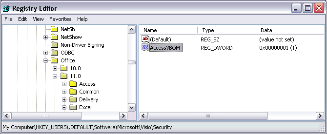
4.1.3 Installing Microsoft Office with Web Components
When installing Microsoft Office Excel not always the Office Web Components get installed. Only in Microsoft Office 2000 the web components are installed during a standard installation. In all other versions, this depends on the type of the Microsoft Office package you are installing and the options selected during the installation. Follow the instructions below when installing Microsoft Excel for the first time. Follow the same instructions when you want to include the Office Web Components after you installed Microsoft Excel.
First Time Installation
Insert the CD-ROM or DVD in your computer and follow the installation instructions. Be certain to select the option to carry out a Custom Installation.
Updating an Existing Installation
Go to the Control Panels via the Windows Start Button and start the Add or Remove Program. From the list of currently installed programs select the version of Microsoft Office (or Excel) that you like to update. Click the Change button.
In the next window select to Add or Remove Features. Click the Next button.
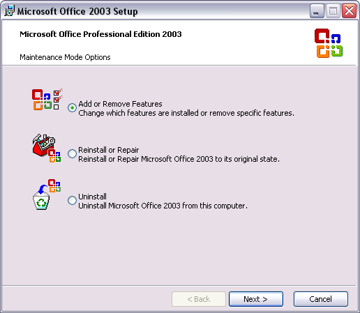
Ensuring Complete Install with Web Components
Now make certain that you have selected the Choose Advanced Customization of Applications checkbox. This is required if you want to carry out a complete install. Click the Next button.
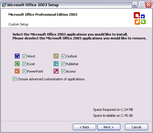
In the list of applications and tools locate Microsoft Office Excel and select the Run all from My Computer option from its pulldown menu (see below). Scroll even further down this list to find the Microsoft Office Shared Tools. Expand this list item, locate Office Web Components and again select the Run all from My Computer option from the associated pulldown. Click the Update button to finish the installation.
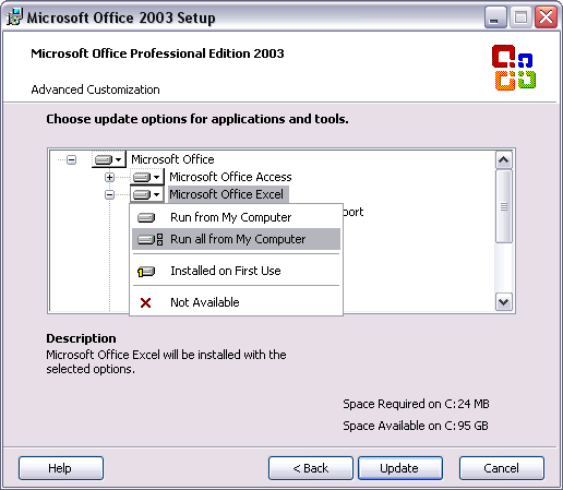
4.1.4 Adding Office Web Components (OWC) after the Microsoft Office Installation
The Degassing Patterns and Import Procedure Blank toolboxes require (and assume) that a recent version of Microsoft Office Web Components have been installed on your computer. In most distributions of Microsoft Office these components are installed, in particular, if you have performed a complete installation of Microsoft Excel. Only in Microsoft Office 2000 the web components are installed during a standard installation. In all other versions, this depends on the type of package you are installing of Microsoft Office and the options selected during the installation (see also: Installing Microsoft Office with Web Components). If the web components are not available, you will be presented with an error message in ArArCALC while trying to display some of the toolboxes with embedded charts.
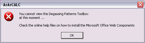
Download the OWC10.exe or OWC11.exe file from one of the appropriate links below to install the web components for Microsoft Office XP or 2003:
Follow the instructions from the Microsoft Download Center web page in order to install the web components on your computer. After the install you should find that the following files have been installed on your computer:
Office 2003
Office XP
Office 2000
Restart Microsoft Excel, which automatically installs the web components.
4.1.5 How to Insert Symbols in Microsoft Excel
When entering data into dialogboxes (for example: Sample Parameters) or when editing your input data in the ArArCALC data tables (see also: Editing Data in ArArCALC), you sometimes need to insert Special Symbols, like the "µ (mu)" or "º (degree)" characters. This is easiest done by applying the Alt+0000 Shortcut Keys as listed below:
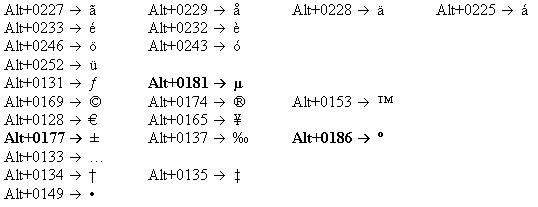
While typing in your text entries, simply hold down the Alt Key and type in the Four Numbers without releasing the alt key. This will insert the required Special Symbol at the place of the cursor. For a complete list of possible Alt+0000 Shortcut Keys please visit http://www-1.ibm.com/support/docview.wss?uid=swg21089251.
4.2 Microsoft Windows 98/2000/XP
This section covers mainly tips on how to perform certain tasks using the Windows platform.
4.2.1 Installing of Fonts
In principle you don't have to install any fonts, except if the V-shaped Flagging Symbols do not appear in your age calculation files (see also: Flagging Analyses in ArArCALC). If that is the case, you need to re-install the "monotype sorts" font:
4.2.2 Working with ArArCALC Diagrams in Adobe Illustrator
Put text here ...
|
|