ArArCALC Help Library |
|||
ArArCALC Help Library |
|||
1.4 Basic ArArCALC Functionality
In this section, the basic steps of ArArCALC are explained, to get you going as quickly as possible. Read this section, in particular, if you're a first-time ArArCALC user. The first part of this section covers How to Start ArArCALC, which Key Settings to define and how to perform Your First Age Calculations. The final part shows you how to Export the age calculations, so that you (or any other user) can read the files directly in Microsoft Excel without running ArArCALC.
1.4.1 How to start ArArCALC from Excel
ArArCALC is easily launched from Microsoft Excel's Tools menu. Note that ArArCALC saves and closes any file already open in Microsoft Excel. It is assumed that ArArCALC is already installed (see also: How to install ArArCALC on your PC).
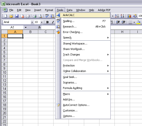
Alternatively, you can start ArArCALC from the Windows Launchbar. To activate this functionality please follow the instructions on the Installing the ArArCALC Icon on the Windows Launchbar help page.
![]()
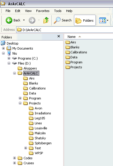
1.4.2 File Organization
ArArCALC has a simply directory structure with six permanent subdirectories: Airs, Blanks, Calibrations, Data, Program and Projects. Note that in the example below ArArCALC has been installed on the "Files (D:)" drive, but in fact ArArCALC can be installed in any (sub)directory and on any drive available on your local system.
The Microsoft Excel Workbooks containing the age calculations are stored in subdirectories of the Projects directory, which are named according to your project name (see also: Managing Irradiations and Projects). Sub-projects are allowed since ArArCALC Version 2.4 and may result in a directory structure like Projects/OJP/Site 1, Projects/OJP/Site 2, etc. However, it is not advisable to add/delete project subdirectories from within the Windows File Manager or Explorer, before making backups of the Projects directory.
The following files are minimally necessary in the Program directory, when executing ArArCALC:
- ArArCALC.age
- ArArCALC.ico
- ArArCALC.log
- ArArCALC.xla
- ArArCALC.xls
- ArArCALC.xlw
Without these files, ArArCALC will terminate its execution.
1.4.3 File Name Conventions
Starting with ArArCALC Version 2.0 this program does not use a default naming convention anymore. The user will simply be prompted to give in Experiment Name and Sample Type when opening a new mass spectrometry data file (see also: Your First Calculation ... How to Start). This gives the user full control on what type of data is being calculated and under which name the *.AGE files are saved in the Projects directories (see also: File Organization). To collate different measurements for an incremental heating experiment into one and the same *.AGE file always use the same Experiment Name and save the files to the same Project directory.

1.4.4 Managing your Irradiations and Projects
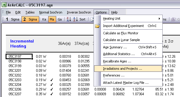
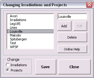
ArArCALC saves all age calculation data files in separate directories according to project name (see also: File Organization). This guarantees an automated and well-structured file organization. However, these project names are logged together with all irradiation parameters in the ArArCALC.log file (see also: Using the ArArCALC.log File). This log file can be accessed and updated through a set of easy-to-use dialogboxes. To activate the Changing Irradiations and Projects dialogbox, select the Options # Irradiation and Projects menu item.
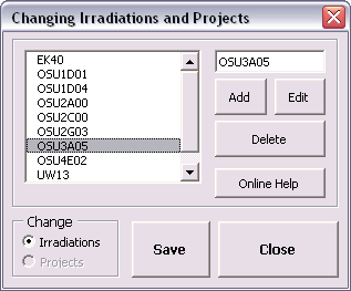
The Changing Irradiations and Projects dialogbox lets you choose what via the option buttons Irradiations and Projects in the lower left Change panel. After making a selection, you can use the Add, Edit and Delete buttons to update either the list of project names or irradiations. To add a new list item, you first need to fill in the name of a new irradiation or project in the textbox in the upper right corner, followed by clicking the Add button. To edit or delete an existing irradiation or project, you first click on its name in the list box, followed by clicking either the Edit or Delete button.
If you want to save your edits, please hit the Save button first, because the Close button will close the Changing Irradiations and Projects dialogbox without saving. If you want to ignore or undo any of your changes, hit the Close button without hitting the Save button first.
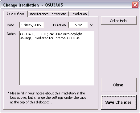
When adding or editing irradiation definitions, ArArCALC will show you the Change Irradiation dialogbox to allow you to define the irradiation parameters, including up to 999 irradiation segments or cycli (see further below).
information
In this tab you can find summary info and notes for a particular irradiation. In here only the Notes can be edited and it is highly recommended that you provide a short description of the irradiation in this field. This description may include which reactor was
used, whether the samples were shielded or not, the purpose of the irradiation, the related project(s) and what time zone was used in the definition of
the Irradiation Cycli or Segments (see below). The Date and Total Duration of the irradiation are automatically calculated from the Irradiation Cycli
data, where the Date represents the first segment listed in the irradiation list and the Total Duration the summed durations as listed in the first column.
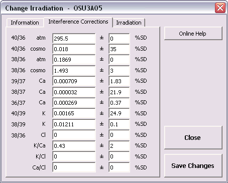
Interference Correction
In this tab you should define the Interference Correction factors and their uncertainties. These constants differ per reactor and whether the samples were shielded or not.
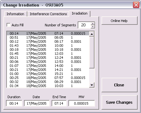
Irradiation segments
In the final tab you can define the Duration, Date, End Time and MW (reactor power) of all Irradiation Cycli or Segments.
It is highly recommended that you use either GMT or your Local Time Zone, as long
as you consistently apply it throughout ArArCALC. For example, you should make certain that you apply the same Time Zone when you define your irradiations and when you supply dates and times in the
Sample Parameters
(see also: Sample Parameters). Use the spin button to increase or decrease the Number of Irradiation Segments. Click on a line in the list box to adjust your settings, which will appear for editing in the
text boxes at the bottom of this dialogbox. To speed up data entry you can also check the Auto Fill option.
1.4.5 Setting your Preferences and Input Filters
The program ArArCALC does not contain any constant in its computer code. Every constant, parameter and setting can be set by the user. This is done to give you 100% control over what you calculate in ArArCALC. Below follows a list of adjustable settings in the Preferences dialogbox.
Isochron Settings
These options let you influence the precision of the YORK2 Isochron calculations (see reference: York, 1969). The Convergence determines how small the difference in slope of the isochron should be for two consecutive iterations to result in a successful least-squared fit. The
Convergence is here expressed as a percentage of the slope itself (see also: Isochron Calculations). The number of Iterations determines after how many iterations the isochron calculation should
be terminated, in case the calculation is not converging. If you set the Convergence to a higher precision (a lower percentage),
you also should adjust the number of Iterations accordingly (to a higher number). Clicking the option button Weighted YORK-2 forces ArArCALC to calculate a least-squared linear fit with correlated errors that is weighted by the inverse of the variance (see
reference: York, 1969). You can overrule this setting when performing isochron calculations by selecting
Normal Isochron # Weighted YORK-2
or Normal Isochron # Unweighted YORK-2 in the menu bar.
You can do the same for the Inverse Isochron independently.
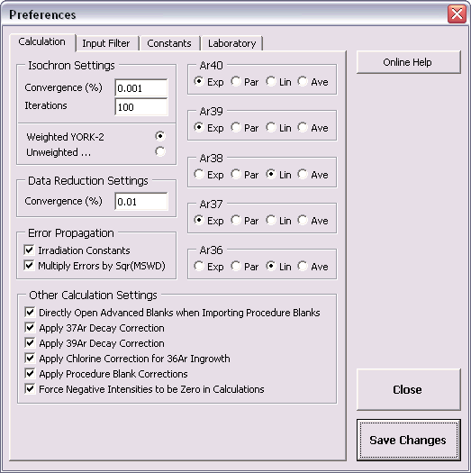
Data Reduction Settings
The data reduction settings determine the precision when you apply the Exponential
Fit to your mass spectrometry data. The Convergence is expressed as a percentage of the curvature coefficient that is iteratively derived in this least-squared fit (see also: Line Fitting).
Error Propagation
By checking Irradiation Constants in the Error Propagation box, the errors on the
irradiation correction factors will be propagated in the reported analytical error (see also: Analytical, Internal and External Errors). You can set these errors in the Change Irradiation dialogbox (see also:
Managing Irradiations and Projects). If the Multiply Errors by Sqr(MSWD) is checked, then the errors on the ages and some isotope ratios (e.g. 40Ar/36Ar and 40Ar/39Ar)
will be multiplied by the sqr(MSWD) in case the MSWD becomes larger than 1 (see also: Analytical, Internal and External Errors). Both options are activated by default in ArArCALC.
Ar40, Ar39, Ar38, Ar37 and Ar36
You can chance the option buttons to the right of the Preferences dialogbox in order to set your Default Calculation Type for the raw data reductions
(see also: Line Fitting). You can do this independently for each isotope by choosing from four calculation types: exponentional (Exp), parabolic or second order
polynomial (Par), linear (Lin) and averaging (Ave). You can always overrule these default settings in ArArCALC when performing the actual line
fits.
Other Calculation Settings
With
these checkboxes you can determine which Additional Corrections to apply (or not apply) during the age calculations (see also: Other Calculation Settings). However, it is always recommended that you apply
the corrections for 37Ar and
39Ar Decay following sample irradiation, for
36Ar Ingrowth in chlorine-rich samples, and for Procedure Blanks.
However, for samples younger than 1 Ma it is recommended that you uncheck the Force Negative Intensities to be Zero
... option. This will allow for more accurate age calculations, because
negative ages (or error bars) are statistically expected and valid for these
kind of samples. ArArCALC will generate a
warning when you select a non-default setting.
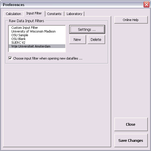
Defining your own Input Filter is most critical while using ArArCALC. Although it may look complicated, it gives you the flexibility to read-in different types of mass spectrometry data files. ArArCALC does not read-in binary files and expects that the measurements were saved in sequentional text files. Furthermore, the actual intensity measurements should be given per line, including the intensity (in volts, amps or counts) and the time (in hours, minutes or seconds) after inlet of the argon gas in the mass spectrometer. By clicking on the Settings button you can define the internal structure of both the header and data sections in a separate dialogbox (see explanation below). By checking the Choose Input Filter when ... checkbox, ArArCALC allows for the selection of an input filter every time you open a new data file. Otherwise the input filter selected in the list box shown below will be used by default.
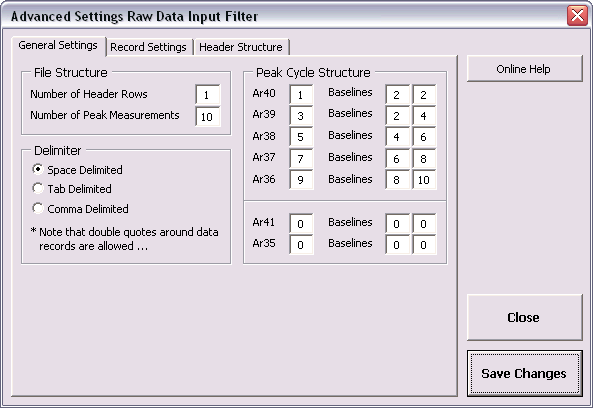
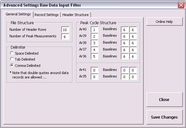
General Settings
The File Structure is determined by the Number of Header Rows and the Number of Peak Measurements for each measurement cycle, and whether the
text file is Space, Comma or Tab delimited. The Number of Peaks should be at least five to cover all five argon peaks between Ar36
and Ar40. In the Peak Cycle Structure the user defines which lines represent
peak measurements for the argon isotopes and which lines represent baseline measurements. These lines can be assigned in random order as long as the Number of Peaks is not exceeded.
If you provide two baseline measurements, ArArCALC calculates an average baseline (see Ar36 through Ar39 below). If you provide one baseline measurement, the baseline value will be
subtracted as is (see Ar40 below). You can also fill in "0" when your data already have been baseline corrected (by your data acquisition software, for example). Two positions for the masses
Ar41 and Ar35
have already been reserved for future importing and monitoring of this data.
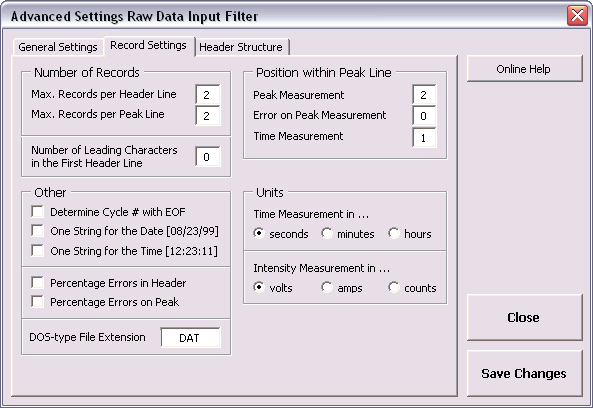
Record Settings
In the
Record Settings tab you can define which records in the peak lines represent the Peak Measurement, the Error on Peak Measurement and the Time Measurement.
Here you can also define in which units the Time
and Intensity Measurements are given and you can define settings such as
the File Extension, the Maximum Number of Records and Header Lines, and how the Date and Time parameters
and the Errors are represented in the
data files. By default
ArArCALC assumes absolute errors.

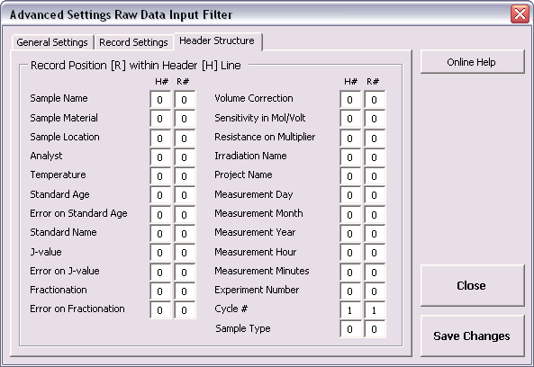
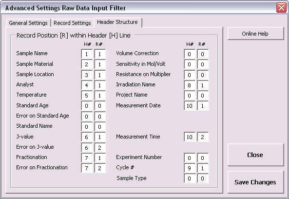
Header Structure
Your raw data files may contain more than 1 header line. In the
Header Structure
tab you can define on which header line (H#) and on which record position (R#) the Sample Name or J-Value was stored. This of
course requires that these headers were originally saved in the data file. In the rather simple example below, only one parameter is stored, namely the Number of Cycli, which is stored in the first record of the first header line. Further below a more
complicated example is shown and explained as well.
Example 1 Space delimited text file 1 header line; 10 peak measurements | |
10 5.76734625000000E-0000 9.06800000000003E+0001 3.50166666666667E-0003 1.01855000000000E+0002 1.61403125000000E-0001 1.18145000000000E+0002 3.44500000000000E-0003 1.33135000000000E+0002 6.75000000000000E-0003 1.43025000000000E+0002 3.48000000000000E-0003 1.52855000000000E+0002 3.16950000000000E-0002 1.62740000000002E+0002 3.45666666666667E-0003 1.73865000000002E+0002 1.01312500000000E-0002 1.90145000000000E+0002 3.39500000000000E-0003 2.06435000000001E+0002 5.64673875000000E-0000 2.17610000000001E+0002 3.51833333333333E-0003 2.28845000000001E+0002 1.60882500000000E-0001 2.45105000000000E+0002 3.44000000000000E-0003 2.60125000000000E+0002 6.74500000000000E-0003 2.70010000000000E+0002 3.56250000000000E-0003 2.79840000000000E+0002 etc. etc. |
The number of cycles Cycle 01; Line 01 = mass 40.0; time in seconds Cycle 01; Line 02 = mass 39.5; time in seconds Cycle 01; Line 03 = mass 39.0; time in seconds Cycle 01; Line 04 = mass 38.5; time in seconds Cycle 01; Line 05 = mass 38.0; time in seconds Cycle 01; Line 06 = mass 37.5; time in seconds Cycle 01; Line 07 = mass 37.0; time in seconds Cycle 01; Line 08 = mass 36.5; time in seconds Cycle 01; Line 09 = mass 36.0; time in seconds Cycle 01; Line 10 = mass 35.5; time in seconds Cycle 02; Line 01 = mass 40.0; time in seconds Cycle 02; Line 02 = mass 39.5; time in seconds Cycle 02; Line 03 = mass 39.0; time in seconds Cycle 02; Line 04 = mass 38.5; time in seconds Cycle 02; Line 05 = mass 38.0; time in seconds Cycle 02; Line 06 = mass 37.5; time in seconds etc. etc. |
This is one of the most simple text files possible (see settings in the dialogboxes displayed above). Its space delimited and it has the minimum amount of headers. The Number of Headers should be set to 1 and consequently the Cycle # should be set to [1,1] as well. Since there is only one header line with only one parameter in it, all other possible header positions should be set to zeros (which is the default value). In this example, each measurement cycle produces 10 individual peak measurements (5 isotopic peaks and 5 baselines) and thus the Number of Peaks should be set at 10. The net peak of Ar40 is calculated based on peak 1 minus the average baseline calculated from peak 2 and peak 2, the net peak of Ar39 is calculated based on peak 3 minus the average baseline calculated from peak 2 and peak 4, etc. etc.
Example 2 Comma delimited text file 10 header lines; 6 peak measurements | |
98Haw001 Plagioclase Deep Canyon Anthony Koppers 1100 0.000345,0.3 1.00038,5.7 VU13 12 19-Mar-1999,14:34:03 5.76734625000000E-0000,9.06800000000003E+0001 1.61403125000000E-0001,1.18145000000000E+0002 6.75000000000000E-0003,1.43025000000000E+0002 3.16950000000000E-0002,1.62740000000002E+0002 1.01312500000000E-0002,1.90145000000000E+0002 3.39500000000000E-0003,2.06435000000001E+0002 5.64673875000000E-0000,2.17610000000001E+0002 1.60882500000000E-0001,2.45105000000000E+0002 6.74500000000000E-0003,2.70010000000000E+0002 etc. etc. |
Sample Name Material Location Analyst Temperature J-value and %SD Fractionation correction factor and %SD Irradiation Name The number of cycles Measurement date and time Cycle 01; Line 01 = mass 40.0; time in seconds Cycle 01; Line 02 = mass 39.0; time in seconds Cycle 01; Line 03 = mass 38.0; time in seconds Cycle 01; Line 04 = mass 37.0; time in seconds Cycle 01; Line 05 = mass 36.0; time in seconds Cycle 01; Line 06 = mass 35.5; time in seconds Cycle 02; Line 01 = mass 40.0; time in seconds Cycle 02; Line 02 = mass 39.0; time in seconds Cycle 02; Line 03 = mass 38.0; time in seconds etc. etc. |
This is a more complicated text file that can be read-in by ArArCALC (see settings in the dialogboxes displayed below). Its comma delimited. It has 10 header lines as is set for the Number of Headers. Each measurement cycle produces 6 individual peak measurements (5 isotopic peaks and 1 baseline at mass 35.5), explaining why the Number of Peaks is only set to 6. The net peak of Ar40 is calculated based on peak 1 minus the average baseline calculated from peak 6 and peak 6 (which is the actual baseline value as measured on mass 35.5), the net peak of Ar39 is calculated based on peak 3 minus the average baseline calculated from peak 6 and peak 6, etc. etc.
The number of cycles can be found on the first record of the 9th header line in this text file and the Cycle # is thus set to [9,1]. The Sample Name, Material, Location and Analyst are all located on the first record of header lines 1 through 4. The Temperature for the measurement is located on header line 5, the J-value and Fractionation Correction Factors and their errors are located on header lines 6 and 7 at records 1 and 2, respectively. The Irradiation Name is located on the first record of header line 8. Finally, the Date and Time are located on header line 10 at records 1 and 2 as well. Since the One String for the Data and Time checkboxes have been selected (see above) only one option is available to you for the Date and Time. If you have them unchecked, you can point to individual values for the Day, Month, Year, Hours and Minutes in the header structure.
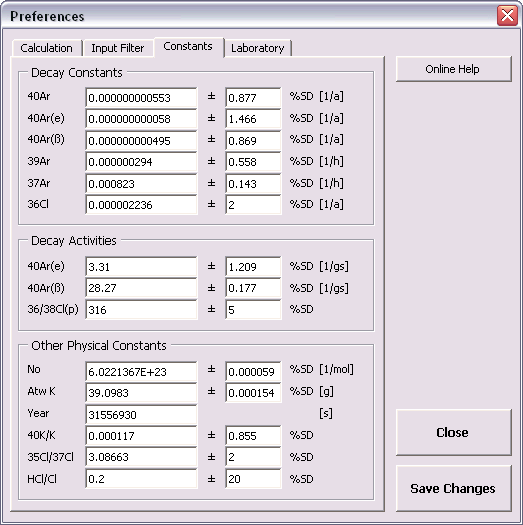
The Decay Constants and their percentual standard deviations can be set and changed in the Preferences dialogbox below. Here you can also define the data for Decay Activities and Other Physical Constants that are needed for the primary age calculations and recalibrations based on the formulations of Karner & Renne (1998), Renne et al. (1998) and Min et al. (2000). For more details read the Primary Age Recalibration Toolbox help page. The expected units are given in the brackets, unless the numbers are dimensionless.
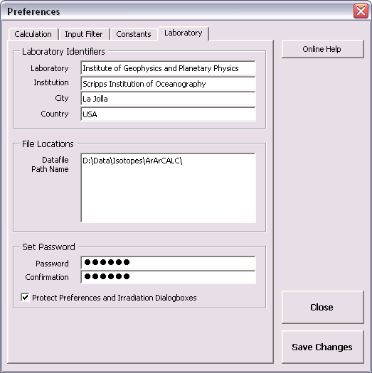
The information you fill out in the Laboratory Identifiers panel will always be printed as headers and footers, next to the date, time and the ArArCALC version number, when you are making a printout from within ArArCALC. You can also set the File Location of the mass spectrometry data files on your hard disk to ensure that ArArCALC swiftly finds your data files. Finally, you may want to set a Password to protect your settings in the Preferences and Irradiation and Project dialogboxes. Setting passwords is, in particular, advised for the person who is managing the Master ArArCALC.log file, in order to circumvent accidental deletion of these important parameters (see also: Using the ArArCALC.log File).
1.4.6 Your First Calculations
Let's assume that ArArCALC is already running (see also: How to start ArArCALC from Excel) and that you have already set your own Project names, Irradiation
Parameters and Preferences (see also:
Managing Irradiations and Projects, Setting the Preferences). Now you are ready to do your first calculation.
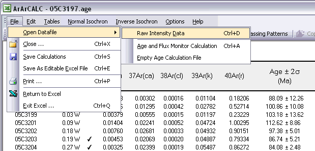
Open a raw intensities data file by selecting the File # Open Datafile # Raw Intensity Data menu item.
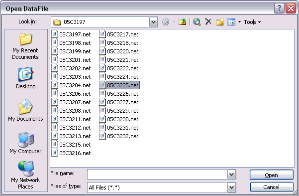
This will give you the following Open DataFile dialogbox. You can set the default file location for these type of data files in the Preferences dialogbox (see: Setting the Preferences) to speed up your file search. Now scroll, select and Open your data file.
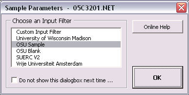
When you open your data file, ArArCALC will show you three dialogboxes in sequence. In the first dialogbox, you have to select an Input Filter. However, you can surpass this dialogbox by unchecking the Choose Input Filter when ... checkbox in the Preferences (see: Setting the Preferences) or by checking the Do not show this dialogbox ... checkbox in the dialogbox shown below. You can use the latter option when you always open your data files with the same input filter.
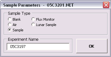
In the second dialogbox, you have to set the Sample Type and give an Experiment Name (See also: File Name Conventions, Sample Type and Experiment Name). When you choose a Blank as the sample type, however, the experiment name is not necessary and thus will be grayed out. To collate different measurements (from different data files) for an incremental heating experiment into one and the same age calculation file, always use the same Experiment Name and save the files to the same Project directory (see next step).
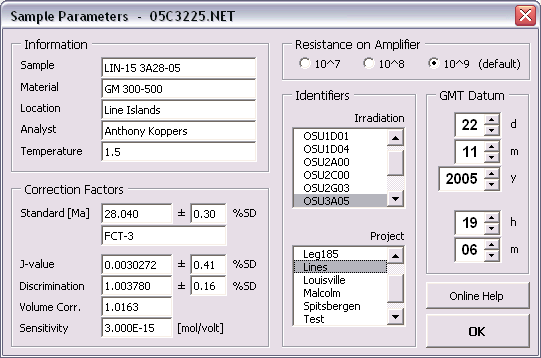
In the final dialogbox, you have to set all Sample Parameters necessary to perform an age calculation. The shown fields are always pre-filled with data from the previous calculation, even if these were performed a few days or weeks ago. Completing this dialogbox will be fast, because most entries will be similar and thus don't need changing when regression data from a single (incremental heating) experiment. Most likely, only the GMT datum and Temperature need editing, unless you start to reduce a totally new experiment. If your raw data files already have header lines containing this information, ArArCALC will automatically transfer this header information into this dialogbox by using your Input Filter (see also: Setting the Preferences). Even in this highly-automated setup this dialogbox will be useful to you, because it allows you to check and edit the sample parameters before further processing of the data commences. You can always recall this dialogbox at a later stage in the Raw Data Reduction view of ArArCALC via the Options # Sample Parameters menu in order to edit the sample parameters.
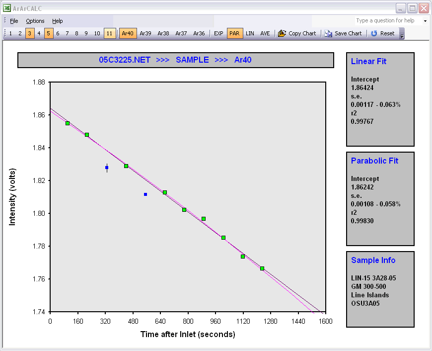
If you have entered all the sample parameters, you will be guided to the Raw Data Reduction view. In this view, a XY-scatter plot displays the measurement time (in seconds) after the inlet of the argon sample in the mass spectrometer on the X-axis, and the intensity of the beam on the Y-axis (in volts, amps or counts). By default, the intensity data for Ar40 is shown first. Each different argon isotope can be calculated by clicking the isotope buttons Ar40, Ar39 ... Ar36. Data points can be included or excluded from the calculations by clicking the toolbar buttons 1, 2, 3, 4 ... 11 that represent the data points, or by clicking the data points themselves on the diagram. Excluded data points are denoted by blue squares and a suppressed toolbar button. The Reset button recalculates including all data points. ArArCALC does not decide which fit to the data (exponentional, parabolic, linear or average) gives the best results. For this purpose, you can set the default regression type for each argon isotope in the preferences (see also: Setting the Preferences). Only in one particular case, when the exponential and parabolic are similar to the linear least-squared fit, ArArCALC accepts a linear fit by default. However, based on the calculation results (see the boxes to the right of the scatter plot) you can always overrule these program decisions yourself, by choosing the appropriate button on the ArArCALC toolbar: Exp, Par, Lin or Ave.
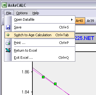
ArArCALC saves all calculated argon intensities of one experiment in one Microsoft Excel 2000-XP-2003 workbook that includes two plateau diagrams and two isochron diagrams, and their respective data tables. The connection between the Raw Data Reduction view (see above) and the Age Calculation view of ArArCALC is easily made through the File # Switch to menu bar item (see also: Switch to ... Option). When you select this option, ArArCALC first saves the calculations and then switches to the age calculation view. You can also make this switch without saving the calculation, by holding down the SHIFT key. If you do not want to switch yet, but you would like to reduce another raw data file, first choose File # Save to save the calculation and then choose File # Open Datafile # Raw Intensity Data to open a new data file.
The following data table will be shown in ArArCALC when you switch to the Age Calculation view. In the shown data table, single incremental heating steps can be excluded or included from the age calculation by double-clicking on the Check Mark symbols. This will automatically recalculate the weighted means, isochrons and other statistics. The Reset button recalculates including all data points. In ArArCALC all errors are calculated as 1 Sigma or 2 Sigma errors. You can report the ages in either the Ka, Ma or Ga age units.
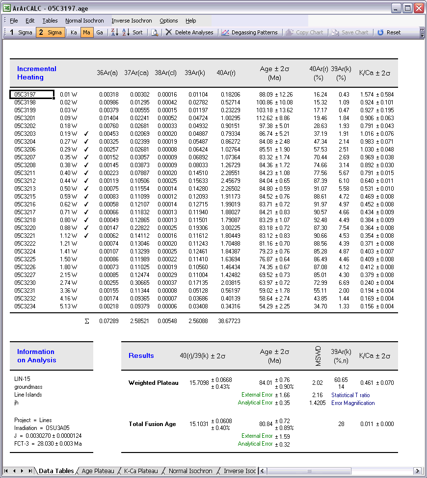
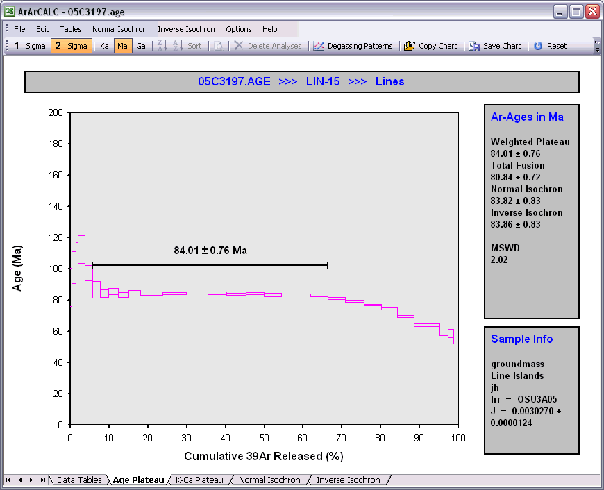
Maneuvering between the different data tables (see also: Selecting Different Data Tables in ArArCALC) and diagrams is simply achieved by clicking the worksheet tabs Data Tables, Age Plateau, K-Ca Plateau, Normal Isochron or Inverse Isochron. Below an example is given for a typical age plateau diagram.
Performing data reductions for Blank and Air Shot measurements starts off the same as for all other measurements. Therefore, the same instructions, as described above, should be followed. ArArCALC saves all reduced blank and air measurements in text files organized per measurement date (blank) or experiment name (air). These files are always stored in the ArArCALC/Blanks and ArArCALC/Airs directories.
1.4.7 Open your Age Calculation in Excel without ArArCALC
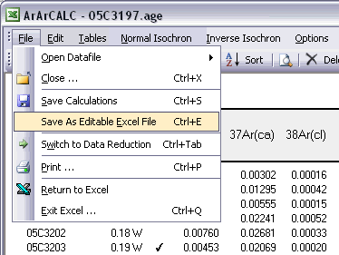
The standard Age Calculation workbooks with the extension *.AGE cannot be opened in Microsoft Excel 2000-XP-2003 without running ArArCALC. These files are password protected to circumvent the possibility of (unexpected) changes made to the workbooks, leaving these files unreadable by ArArCALC itself. However, if you save your calculations via the File # Save as Editable Excel File (Ctrl+E) option, the password protection and the Microsoft Excel macros are removed. Now you can open these newly-saved files with the extension *.XLS in Microsoft Excel and change the format of their data tables and diagrams manually. A progress bar appears, showing you the status while saving these editable files.
See also ...
Contents ArArCALC Chapter 1 Using ArArCALC Section 1.1 Key Information Section 1.2 Getting Help Section 1.3 Installing and Removing ArArCALC Section 1.5 Navigating and Flagging Data Points