2.3  Age Calculations

Functions specific to the Age Calculation view will be discussed in this section. Saving, exporting and closing age calculations files all are done from the File menu, while many advanced (calculation) functions are available from the Options menu. You can use the Edit and Table menus to navigate between the nine data tables in which ArArCALC stores your data, and you can use the Normal and Inverse Isochron menus to set your preferences for the isochron calculations and their display options.

2.3.1  Close

Select the File # Close (Ctrl+X) menu item to Close the active age calculation file. In all cases your age calculation file will be saved upon closing (even though no progress bar is shown).

2.3.2  Save Calculations

To Save your calculations select the File # Save Calculations (Ctrl+S) menu item. This also will save your user preferences, calculation settings and irradiation definitions, as they are stored in your age calculation file. During saving the latest ArArCALC Version Number is added to the properties of the file itself, which you can view by selecting the File Properties within Windows Explorer. A progress bar appears, showing you the status while saving.

2.3.3  Export for Publication

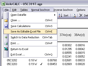
The standard Age Calculation workbooks with the extension *.AGE cannot be opened in Microsoft Excel 2000-XP-2003 without running ArArCALC. These files are password protected to circumvent the possibility of (unexpected) changes made to the workbooks, leaving these files unreadable by ArArCALC itself. However, if you save your calculations via the File # Save as Editable Excel File (Ctrl+E) option, the password protection and the Microsoft Excel macros are removed. Now you can open these newly-saved files with the extension *.XLS in Microsoft Excel and change the format of their data tables and diagrams manually. A progress bar appears, showing you the status while saving these editable files.

2.3.5  Switch to Data Reduction

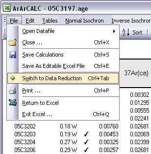
Switching from the Age Calculation view to the Raw Data Reduction view is very simple. To do so, you should select the File # Switch to Data Reduction (Ctrl+Tab) menu option.

2.3.6  Edit Menu

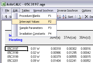
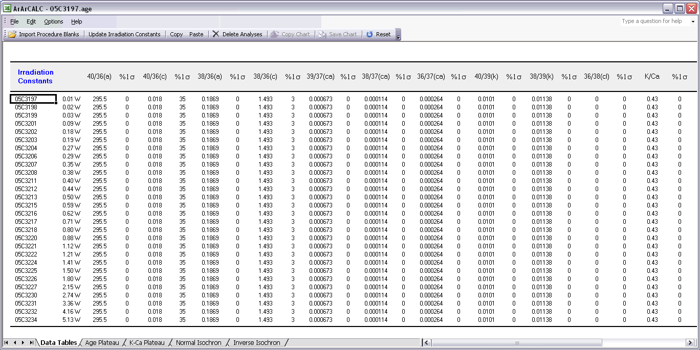
Four data tables in ArArCALC include data necessary for the age calculations, but which you always can edit. These data tables are all located in the Data Tables worksheet and can be selected through the Edit menu. You can also use the F1, F2, F3 and F4 keyboard strokes for faster navigation between these tables.

Procedure Blanks

ArArCALC has been set-up to run on-line during mass spectrometry and by default uses the latest-calculated blank measurement for its blank corrections. However, you can always edit the blank intensities later via the Edit # Procedure Blanks menu item. This function displays a data table containing Blank Intensities and their 1σ Standard Error (SE) for each analysis (step) in your (incremental heating) experiment. You can edit these blank data by clicking the cells and typing in new values. A single click lets you replace the complete number, whereas double-clicking will allow you to edit the number within its cell. To copy values from one cell to another, use the Drag functions of Microsoft Excel (drag the black square anchor visible on the highlighted cell down or to the right) or use the Copy (Ctrl+C) and Paste (Ctrl+P) buttons. Note that you can also copy blank values via the clipboard, in which case you select the cells in which to place your new values and use the Paste (Ctrl+P) button. The Reset button will undo all edits, unless you already have saved them.

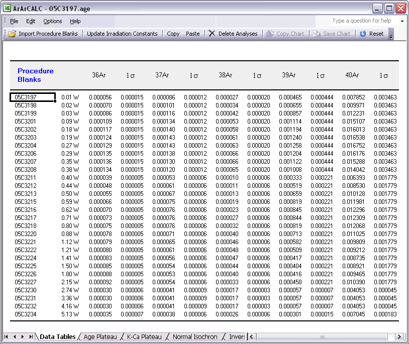
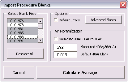
You can also select single (or multiple) cells, representing one (or more) analyses, and then choose Import Procedure Blanks from the toolbar. Since ArArCALC saves all blank measurements in text files organized per measurement date, this function allows you to import multiple blank measurements for a range of days, by opening more than one of these text files. Blank measurements can now be selected in the Select Blank Files list box to calculate Average Blanks for all argon isotopes, including their (predicted) standard deviations. This ArArCALC tool then automatically replaces all blank values and uncertainties in the edit table for the selected analyses. However, when the Default Errors checkbox is checked, the standard deviations will be overruled by percentual errors.

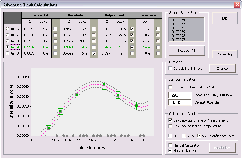
You can also click the Advanced Blanks button to analyze the Evolution in the Procedure Blanks over the same range of days. For each argon isotope you can now calculate a linear, parabolic or polynomial fit (pink dashed line). These calculations can be done while generating a standard error or 65-95% confidence envelop (grey dashed lines). The unknowns for which to calculate the blank values are indicated by gray circles at the bottom of the diagram (see also: Import Procedure Blank Toolbox). When you click the OK button, this ArArCALC tool again replaces all blank values and uncertainties in the edit table for the selected analyses.

Intercept Values

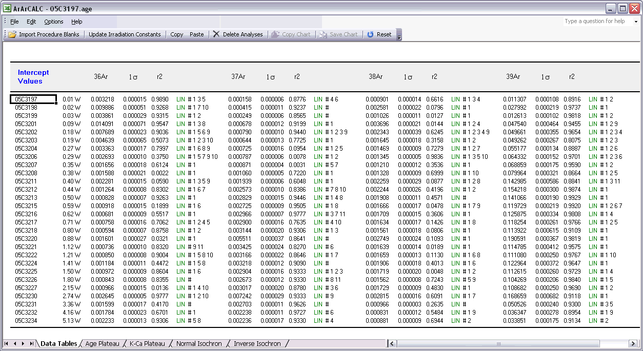
You can edit the intercept values via the Edit # Intercept Values menu item. In this data table all Intercept Values including their 1σ Standard Error (SE) are stored together with the r², the type of line fit (EXP, PAR, LIN or AVE) and the data points excluded from the data regression. Editing is similar as described above. The Reset button will undo all edits.

Sample Parameters

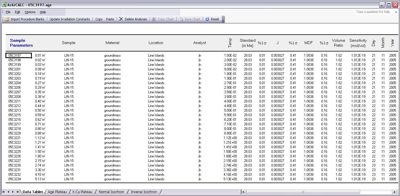
The Sample Parameters (see also: Your First Calculations, Sample Parameters) can be edited via the Edit # Sample Parameters menu. This offers you the possibility to later finalize the actual J-value used in the age calculations or to better define the timing of the measurements. Note that in all the data tables the first two columns on the left (analyses number and increment temperature) cannot be edited. Although there is no possibility (and no need) to edit the analyses numbers, you always can adjust the temperature for each incremental heating step or analysis in the Temp column. All other values can be edited manually. The Reset button will undo all edits.

Irradiation Constants

Finally, the Irradiation Constants may be edited via the Edit # Irradiation Constants menu item. This makes possible the combined age calculation of samples with different irradiation histories (see also: Import Additional Experiments). All irradiation constants can be edited manually. They can also be updated in one go by clicking the Update Irradiation Constants button, which will replace all values with the latest values found in the ArArCALC.log file (see also: Update Irradiation Constants). If you are going to calculate ages in the lunar mode, the labels of this table automatically will be changed from 40/36(a) to 40/36(t) and a default value of 40/36(t) = 1 is assumed (see also: Calculate as Lunar Sample). When you toggle back to the terrestrial age calculation mode, this value gets reset to the default 295.5 value for atmospheric argon. These are the only hard-coded values in ArArCALC and only are applied when toggling to lunar age calculations and back, but you always can overwrite these values by editing the Irradiation Constants table again. The Reset button will undo all edits.

2.3.7  Tables Menu

Nine different data tables are available in every ArArCALC age calculation file. Five of these tables include output data from your age calculations, whereas four tables include the input data necessary to perform the age calculations and which you can edit at any time (see also: Editing Data in ArArCALC). The calculation data tables are all located in the Data Tables worksheet and are selectable through the Tables menu. You can also use the F5, F6, F7, F8 and F9 keyboard strokes for faster navigation between the tables.

Age Plateau

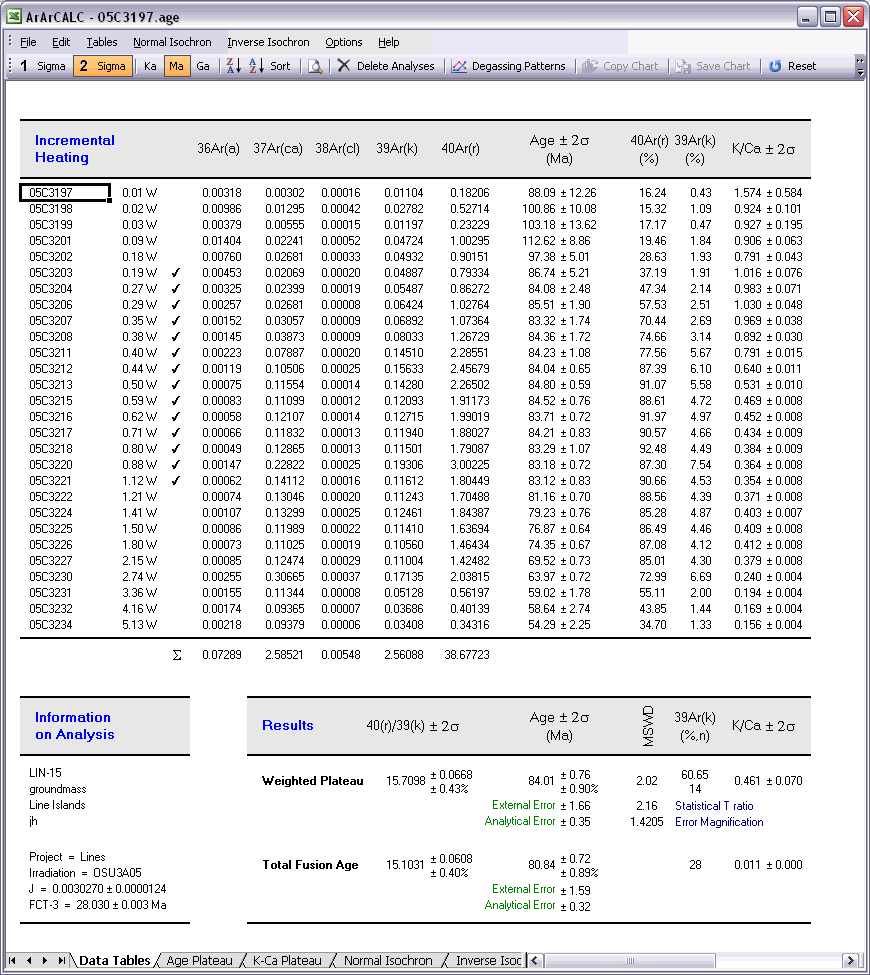
The Age Plateau data table contains calculation data for the plateau age, total fusion ages and K/Ca ratios. Note that also the MSWD, the number of increments and the total amount of ³⁹Ar(k) in percent are given for the age plateau calculation. The uncertainties on the ⁴⁰Ar/³⁹Ar ages are defined as Internal Errors that combine the Analytical Errors with the Errors on the J-value. For completeness, the Analytical Errors and External Errors (including the error on the total ⁴⁰Ar decay constant) are given as well (see also: Analytical, Internal and External Errors). The checkmarks signify the analyses included in the age plateau calculation, whereas the summed ³⁶Ar(a), ³⁷Ar(ca), ³⁸Ar(cl), ³⁹Ar(k) and ⁴⁰Ar(r) components at the bottom of the table are used to calculate the total fusion (or recombined) age.

Isochrons

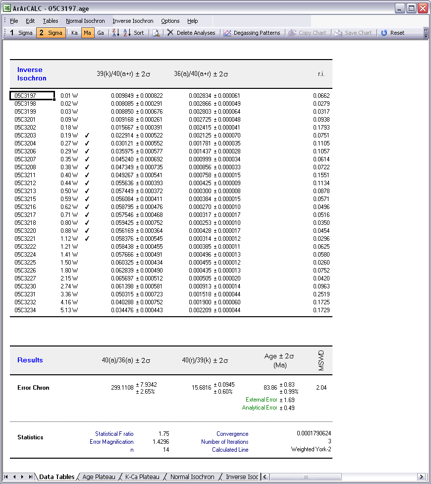
The Normal Isochron and Inverse Isochron data tables contain the calculated ratios ³⁹Ar/³⁶Ar, ⁴⁰Ar/³⁶Ar, ³⁹Ar/⁴⁰Ar and ³⁶Ar/⁴⁰Ar as used in the York (1969) isochron calculations. Both tables display correlation coefficients (r.i) denoting to what extend the errors used in these isotope ratios are correlated. In the example of an inverse isochron below, the correlation is minimal, because the error in the ⁴⁰Ar (denominator) is small compared to the errors on ³⁹Ar and ³⁶Ar (the nominators). In the Statistics section the isochron calculations are further described by the convergence, number of iterations, type of calculated line, F-ratio, error magnification factor, and the number of points included in these calculations.

Degassing Patterns

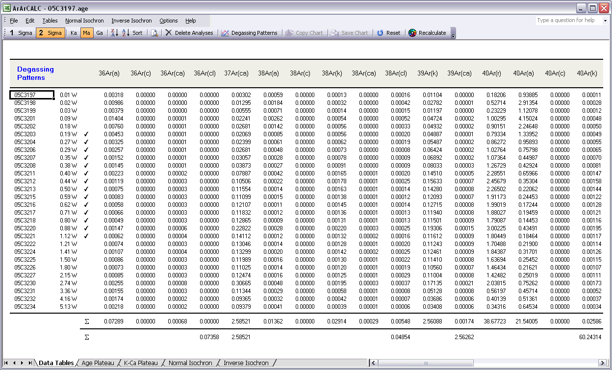
The Degassing Patterns data table contains for every analyses in your experiments the calculated argon components. For example, the entire measurement for the ³⁶Ar isotope can be divided into the ³⁶Ar(a) atmospheric, ³⁶Ar(ca) calcium and ³⁶Ar(cl) chlorine components, and if you are analyzing lunar rocks, also the ³⁶Ar(c) cosmogenic component. For each individual component all increments or steps are summed, while the components themselves are summed as well (see the bottom of the table). A selection of these summed components appears in the Age Plateau data table as well (see above) and they are used to calculate the total fusion ages or to display these in the isochron diagrams (see also: Total Fusion Points in Isochron Diagrams). You can also visualize the Degassing Patterns in an interactive toolbox (see also: Degassing Patterns Toolbox).

Additional Parameters

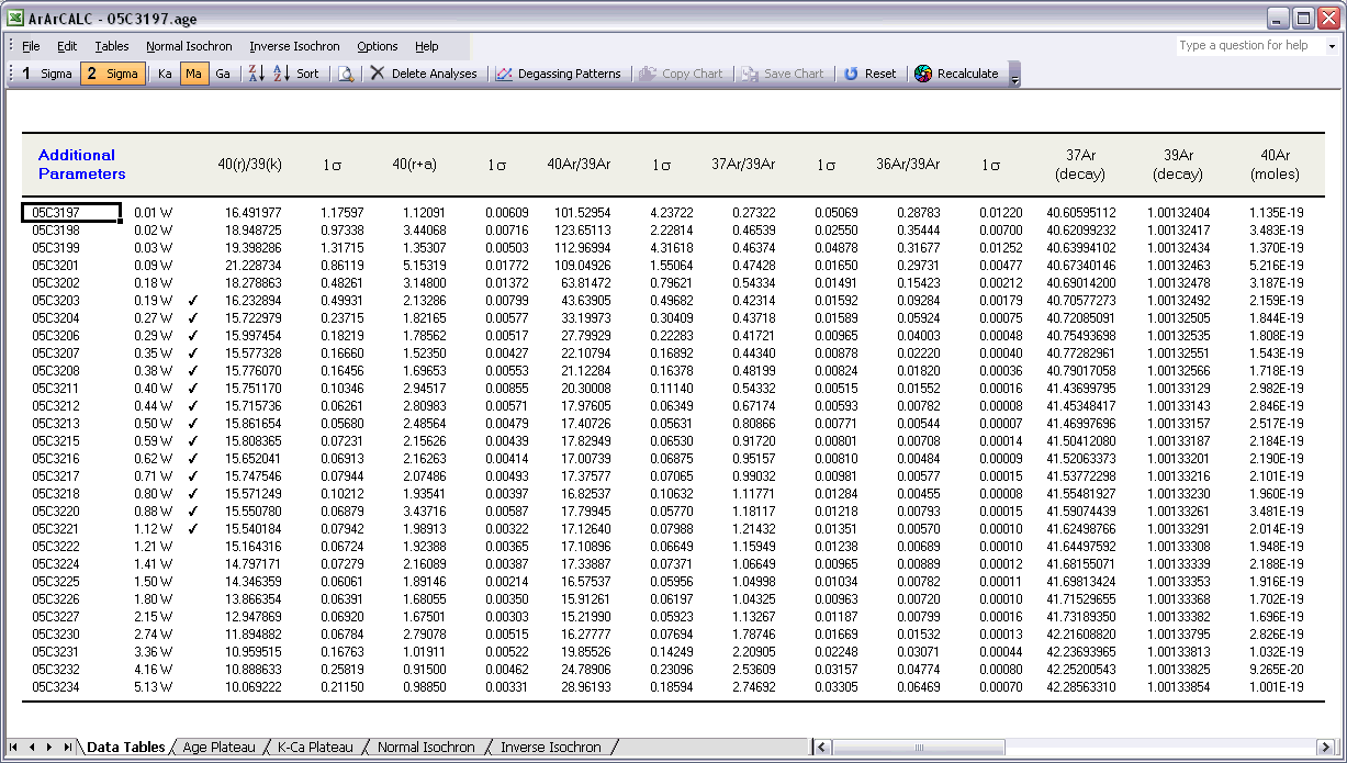
The last data table for Additional Parameters contains an extra selection of data that may be interesting to you when judging the outcome of your argon experiments. Most notable are the decay correction factors for ³⁷Ar and ³⁹Ar, which are used to correct for radioactive decay occurring between the irradiation of the sample and your actual measurements. But also the absolute amount of ⁴⁰Ar measured is listed here in moles, and the corrected ⁴⁰Ar/³⁹Ar, ³⁷Ar/³⁹Ar and ³⁶Ar/³⁹Ar ratios and their uncertainties.

2.3.8  Normal and Inverse Isochron Menus

Individual menus are available for the Normal and Inverse Isochrons, allowing you to change a variety of Display options for each isochron separately and to toggle the calculations between Weighted/Unweighted YORK-2 Fits.

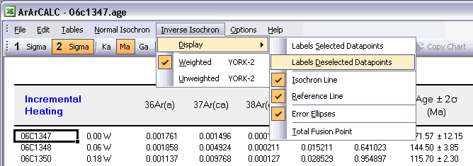
Display Labels for Selected Data Points

You can show or hide Labels for the Selected data points (green squares) in your isochron diagrams by toggling this menu item. The labels always show you the Temperature for a specific (incremental heating) data point. For example, 0.06W or 1500°C.

Display Labels for Deselected Data Points

Alternatively, you can show or hide the same Temperature Labels for the Deselected data points (blue squares).

Display Isochron Line

With this menu item you can show or hide the calculated Isochron line (pink line). The isochron line is shown by default, except if less than 3 data points are included in the calculations.

Display Reference Line

You can also show or hide the Reference line (dark grey line) that depicts the line between the Plateau Age Intercept on the ³⁹Ar/⁴⁰Ar axis and the Atmospheric Argon Intercept (295.5) on the ³⁶Ar/⁴⁰Ar axis. In a perfect case, the reference and isochron lines overlap on the 95% confidence level. The reference line is shown by default, except if less than 3 data points are included in the calculations.

Display Error Ellipses

To show or hide Error Ellipses in the isochron plots toggle this menu item. Since the ratios on the axes of the isochron diagrams have errors that are correlated, the ellipses always become (slightly) inclined. This is more clear in normal isochrons than in inverse isochrons, where in the normal isochron diagrams the ellipses often get elongated extensively and rotated to line up with the isochron itself. In that case, it is often easier to hide the error ellipses from view, which also is the default setting in ArArCALC for normal isochrons. For the inverse isochrons, the ellipses are shown by default.

Display Total Fusion Point

The Total Fusion Point (red circle) can be shown or hidden in both isochrons. By default ArArCALC shows this point, because in a closed system, this point is expected to coincide with (i.e. falling on) the isochron line. These points thus provide you with an easy visual check on this particular characteristic for your sample.

Apply Weighted YORK-2 Fit

By default the Isochron calculations are performed using Weighted Errors (York, 1969).

Apply Unweighted YORK-2 Fit

In some cases, you might want to use an Unweighted YORK-2 Fit. A good example is, if one of your data points has an unusual small error (because you employed a too large incremental heating step) and thus (unrealistically) outweighs all other data points in your isochron calculations. By choosing this option, a linear fit without any weighting gets performed, and thus ignores the unevenness in your heating schedule.

2.3.9  Heating Unit

You can set the Heating Unit for your sample to either Laser Wattage, Laser % or Temperature (in °C). Simple select your option from the Options # Heating Unit menu item, and the tables in ArArCALC will automatically be updated and reformatted.

2.3.10  Import Additional Experiment

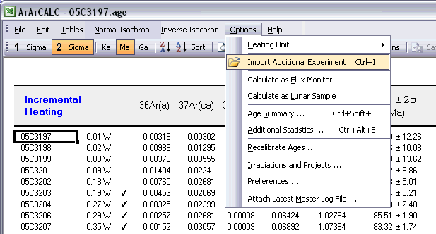
You can also Combine Multiple Experiments in single ArArCALC age calculation workbooks, when using the Options # Import Additional Experiment menu item. This functionality allows you to combine analyses from co-magmatic mineral separates (e.g. plagioclase and hornblende) from one rock sample into a single isochron calculation. Also, multiple total fusion experiments for one flux monitor standard can be merged into one calculation. Finally, this functionality allows you to combine or directly compare sample splits measured in different laboratories or from different irradiations.

2.3.11  Calculate as Flux Monitor

Choosing the Options # Calculate as Flux Monitor menu item toggles between calculation of J-values and ages. This is possible since ArArCALC requires the input of both the standard age and J-value (and their uncertainties) for every analysis (see also: Your First Calculation ... How to Start). This functionality may be useful to you, when you are reducing data from flux monitor standards, for which both the resulting standard age and J-value are of interest.

2.3.12  Calculate as Lunar Sample

Choosing the Options # Calculate as Lunar Sample menu item toggles between calculation of terrestrial and lunar ages. When calculating Lunar Ages the atmospheric component is replaced with a trapped component and an additional cosmogenic component is added into your calculations.

2.3.14  Display Additional Statistics

Choosing the Options # Additional Statistics menu item displays a dialogbox containing a summary of the plateau age (or J-value), plus a list of additional statistical parameters describing the shape and form of the plateau itself. The perfect (flat) age plateau would have a slope and skewness of zero, a high positive kurtosis and a low square of deviations.

2.3.20  Attach Latest Master Log File

In some cases, you may want to replace the log files that are attached to your age calculation files with the latest Master ArArCALC.log file. Select the Options # Attach Latest Master Log File menu item. First the old log files will be removed from your Excel workbook, where after a copy of the latest master settings will be appended again (see also: Using the ArArCALC.log File). Before replacing the log files, you will be asked to confirm this action.

2.3.22  Ka, Ma and Ga Buttons

You can report your age data either in Ka, Ma or Ga units. Click the appropriate button in the ArArCALC Toolbar and your data will be recalculated and reformatted accordingly. Ma is the default setting in ArArCALC.

2.3.23  Table Sorting

You can sort the data tables by selecting any cell in the column on which you like to sort and then hit one of the Sort buttons. The sort can be performed in a descending (first button) or ascending (second button) order. You can sort using up to three different sorting keys. To use more than one sorting key, you should select up to three different cells in three different columns while holding down the CTRL button and then hit one of the Sort buttons. To restore the default sorting order, you should sort on the first column, as shown in each table, or on the temperature column in case of an incremental heating experiment.

2.3.24  Table Zooming

You can Zoom In on the text in the data tables by clicking on the Magnification Glass button in the ArArCALC Toolbar. To restore the view, select the 100% zoom level after clicking the Magnification Glass button again.

2.3.25  Delete Analyses

You can always delete analyses from your age calculation files. Simply select one or more analyses in the data table and click Delete Analyses on the ArArCALC Toolbar. You will be asked to confirm the deletion.

2.3.26  Degassing Patterns Toolbox

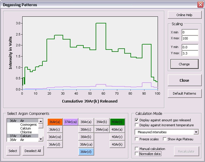
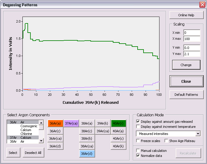
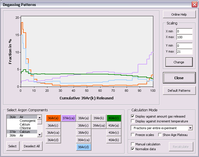
The degassing of whole rock and basaltic groundmass samples during incremental heating experiments can be rather complex (for example Koppers et al. 2000 and 2004). The Degassing Patterns Toolbox is provided to you to better study and understand these degassing behaviors. In the example below of a submarine groundmass sample, the measured intensities of four argon components are shown, as indicated by the orange, purple, light blue and green buttons in the Select Argon Components panel. This is an interesting view of the degassing behavior of this sample, but the signal is rather erratic and the high intensity for the ⁴⁰Ar(r) Component forces the other components to be nearly invisible near the bottom axis. This view becomes much more useful, if we normalize the signal (i.e. intensity) to the step size, as shown in the second example below. The ⁴⁰Ar(r) Component now closely resembles the shape of the age spectra, which is what we are expecting, yet its intensity still overwhelms the other components. This problem gets alleviated as well, if we plot the degassing patterns as fractions over the entire experiment. This is shown in the third example below and clearly brings forward the low intensity components in the same plot. As it turns out, this experiment shows large spikes in the ³⁶Ar(a) and ³⁸Ar(cl) Components for the low temperature increments and another spike in the ³⁷Ar(ca) Component for the high temperature increments. These are very useful observations that will help you in the interpretation of complex argon age spectra.

Select Argon Components
To select or deselect certain Argon Components, click either on the buttons or make your selections in the list box on the left-hand side. You can also use the buttons beneath this list box to Select All or Deselect All. The colors of the selected buttons correspond to the colors of the lines in the diagram.

Calculation Mode
By default the data are plotted against the Cumulative Amount of ³⁹Ar(k) Released. However, you can also display the data against the Increment Temperature in case of a incremental heating experiment. Select one of the two checkboxes to change between these modes. Freeze Scales is helpful when you want to save the scaling settings between different toolbox sessions. You can also select the Show Age Plateau checkbox, which will add a horizontal bar to the plot, indicating the position of the age plateau. Check the Normalize Data checkbox if you want the normalize the intensities measured against the step size or the amount of ³⁹Ar(k) in each increment. And, finally, you can disable the automatic updating of the plot and do a Manual Calculation. In that case use the Recalculate button to update the calculations.

Scaling
To manually scale the plot, change the numbers in the Scaling panel and click on the Change button. If you want to retain these customs settings between different toolbox sessions, be certain to check the Freeze Scale checkbox.

2.3.27  Copy Chart

To use or edit your plateau and isochron diagrams in your favorite drawing program, click the Copy Chart button on the ArArCALC Toolbar. Your diagrams will be put onto the clipboard in a vector graphics format and can be pasted straight into software tools like Adobe Illustrator, Canvas or CorelDraw (see also: Working with ArArCALC Diagrams in Adobe Illustrator).

2.3.28  Save Chart

You can also save your plateau and isochron diagrams as a GIF Image by clicking the Save Chart button on the ArArCALC Toolbar. The image files will be saved automatically in your Project folders (see also: File Organization).

2.3.29  Reset

By clicking the Reset button on the ArArCALC Toolbar you will include all "unflagged" analyses in your calculations again. Upon calculation all tables and diagrams will be updated accordingly (see also: Flagging Analyses in ArArCALC).

2.3.30  Recalculate

Click the Recalculate button on the ArArCALC Toolbar if you want to refresh the age calculations. In most cases, this is not necessary, because ArArCALC automatically recalculates the ages when you make changes. There is one exception, however, that is when you have updated your preferences or irradiation constants (see also: Preferences, Irradiations and Projects). In that case, your new settings will be applied when you hit the Recalculate button or when ArArCALC recalculates because you made other changes to the age calculation file. Examples of the latter are the (un)flagging of your analyses, adding or deleting analyses, changing the 1 or 2 sigma confidence level, changing the age units, etc.

See also ...

Contents	ArArCALC
Chapter 2	Function by Function
Section 2.1	General Functions
Section 2.2	Raw Data Reduction
Section 2.5	Editing Mode

	First  |  Previous  |  Next  |  Last