Standard Paleointensity Definitions

The index

$i$ is used to denote the

$i^{th}$ temperature step of the paleointensity experiment.

$i$ is used to index Arai plot data (e.g.,

$x_i$ , or

$y_i$ ) and ranges from

$i=1$ to

$n_{max}$ , where

$n_{max}$ is the total number of steps on the Arai plot.

$start$ and

$end$ denote the

$i$ indices of the selected steps used for analyzing the paleointensity results.

$i=start$ denotes the first selected data point and

$i=end$ denotes the last.

The number of points on an Arai diagram used to estimate the best-fit linear segment and the paleointensity (

$n=end-start+1$ ).

3.2 The paleointensity estimate

The slope of the best-fit line of the selected TRM and NRM points on the Arai plot. Determination of the slope uses the standardized major axis form of least squares linear fitting (York, 1966; Coe et al., 1978).

$b=\textrm{sign} \left\{ \sum\limits_{i=start}^{end}{(x_i-\bar{x})(y_i-\bar{y})}\right\}\left(\frac{\sum\limits_{i=start}^{end}{(y_i-\bar{y})^2}}{\sum\limits_{i=start}^{end}{(x_i-\bar{x})^2}}\right)^{\frac{1}{2}},$ where

$\bar{x}$ and

$\bar{y}$ are the mean TRM and NRM values of the data selected for the best-fit, that is,

$\bar{x}=\frac{\sum\limits_{i=start}^{end}{x_i}}{n},$ and

$\bar{y}=\frac{\sum\limits_{i=start}^{end}{y_i}}{n}.$

The standard error on the slope is given by:

$\sigma_b=\left(\frac{2\sum\limits_{i=start}^{end}{(y_i-\bar{y})^2} -2b \sum\limits_{i=start}^{end}{(x_i-\bar{x})(y_i-\bar{y})}} {(n-2)\sum\limits_{i=start}^{end}{(x_i-\bar{x})^2}}\right)^{\frac{1}{2}}$

Useful Note...
It should be noted that the standard line-fitting routines available in most analysis software (e.g., Excel) do not use the standardized major axis fitting routine, but instead use linear regression (sometimes known as ordinary least-squares), whereby only the y-axis residuals are minimized. Given that accurate estimation of the slope is the objective of paleointensity analysis, standardized major axis, as outlined above, is the most appropriate method (e.g., Warton et al., 2006).

Statistic: $B_{Anc}$ and $\sigma_B$ , the paleointensity estimate and its error
Report to 1 d.p.

A paleointensity estimate is obtained from

$B_{Anc}=\left|b\right|\times{}B_{Lab}$ , where

$B_{Lab}$ is the strength of the laboratory field. The associated standard error of the estimate is given by

$\sigma_{B}=\sigma_{b}\times{}B_{Lab}$ .

3.3 Arai plot statistics

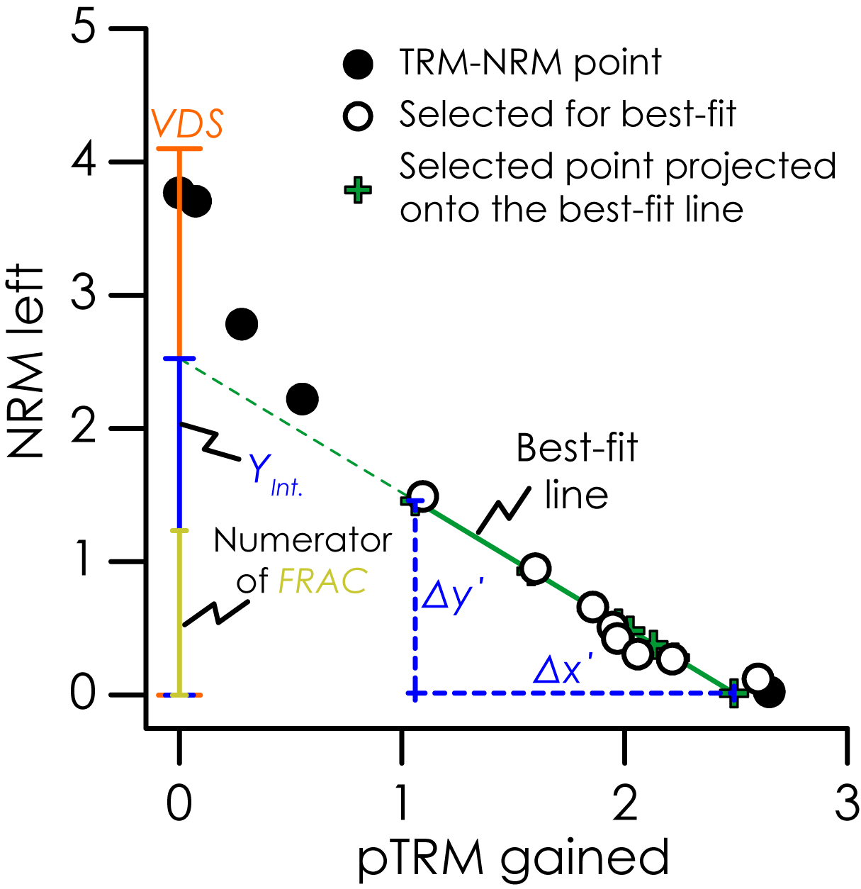
The y-axis (NRM) intercept of the best-fit line on the Arai plot.

$Y_{Int.}=\bar{y}-b\bar{x}$

The x-axis (TRM) intercept of the best-fit line on the Arai plot.

$X_{Int.}=\frac{-Y_{Int.}}{b}$

The vector difference sum of the entire NRM vector (

$\mathbf{NRM}$ ).

$VDS=\left|\mathbf{NRM}_{n_{max}}\right|+\sum\limits_{i=1}^{n_{max}-1}{\left|\mathbf{NRM}_{i+1}-\mathbf{NRM}_{i}\right|},$

where

$\left|\mathbf{NRM}_{i}\right|$ denotes the length of the NRM vector at the

$i^{th}$ step.

$x'$ and

$y'$ the

$x$ and

$y$ points on the Arai plot projected on to the best-fit line. These are used to calculate the NRM fraction and the length of the best-fit line among other parameters. There are multiple ways of calculating

$x'$ and

$y'$ , below is one example.

$x'_i=\frac{1}{2}\left(x_i+\frac{y_i-Y_{Int.}}{b}\right)$

$y'_i=\frac{1}{2}\left(y_i+bx+Y_{Int}\right)$

$\Delta{x'}$ and

$\Delta{y'}$ are TRM and NRM lengths of the best-fit line on the Arai plot, respectively (Figure 1).

$\Delta{x'}=\left|[\max{\{x'_i\}} - \min{\{x'_i\}}]_{i=start, \ldots, end}\right|$

$\Delta{y'}=\left|[\max{\{y'_i\}} - \min{\{y'_i\}}]_{i=start, \ldots, end}\right|$

NRM fraction used for the best-fit on an Arai diagram (Coe et al., 1978).

$f=\frac{\Delta{y'}}{\left|Y_{Int.}\right|}$

NRM fraction used for the best-fit on an Arai diagram calculated as a vector difference sum (Tauxe and Staudigel, 2004).

$f_{VDS}=\frac{\Delta{y'}}{VDS}$

NRM fraction used for the best-fit on an Arai diagram determined entirely by vector difference sum calculation (Shaar and Tauxe, 2013).

$FRAC=\frac{\sum\limits_{i=start}^{end-1}{ \left|\mathbf{NRM}_{i+1}-\mathbf{NRM}_{i}\right| }}{VDS}$

$\beta$ is a measure of the relative data scatter around the best-fit line and is the ratio of the standard error of the slope to the absolute value of the slope (Coe et al., 1978)

$\beta=\frac{\sigma_b}{\left|b\right|}$

The gap factor (

$g$ ) is a measure of the average NRM lost between successive temperature steps of the segment chosen for the best-fit line on the Arai plot. The gap reflects the average spacing of the selected Arai plot points along the best-fit line.

$g=1-\frac{\sum\limits_{i=start}^{end-1}{\left(y'_{i+1}-y'_i\right)^2}} {\Delta{y'}^2}.$

The upper limit of

$g$ is dependent on

$n$ and occurs when the points on the Arai plot are evenly spaced.

$g_{lim}=\frac{n-2}{n-1}.$

The gap factor defined above is measure of the average Arai plot point spacing and may not represent extremes of spacing. To account for this Shaar and Tauxe (2013)) proposed

$GAP\textrm{-}MAX$ , which is the maximum gap between two points determined by vector arithmetic.

$GAP\textrm{-}MAX=\frac{\max{\{\left|\mathbf{NRM}_{i+1}-\mathbf{NRM}_{i}\right|\}}_{i=start, \ldots, end-1}}{\sum\limits_{i=start}^{end-1}{\left|\mathbf{NRM}_{i+1}-\mathbf{NRM}_{i}\right|}}$

The quality factor (

$q$ ) is a measure of the overall quality of the paleointensity estimate and combines the relative scatter of the best-fit line, the NRM fraction and the gap factor (Coe et al., 1978).

$q=\frac{\left|b\right|fg}{\sigma_b}=\frac{fg}{\beta}$

Weighting factor of Prévot et al. (1985).

$w=\frac{fg}{s},$ where

$s^2$ is given by:

$s^2=2+\frac{2\sum\limits_{i=start}^{end}{(x_i-\bar{x})(y_i-\bar{y})}}{\left( \sum\limits_{i=start}^{end}{(x_i-\bar{x})^{\frac{1}{2}}} \sum\limits_{i=start}^{end}{(y_i-\bar{y})^2} \right)^2}.$ It can be noted, however, that

$w$ can be more readily calculated as:

$w=\frac{q}{\sqrt{n-2}}.$

The curvature of the Arai plot as determined by the best-fit circle to all of the data (Paterson, 2011). To determine the Arai curvature, a best-fit circle of the form

$(x-a)^2 + (y-b)^2 = r^2$ is fitted to all of the data using a least-squares approach. For the fitting process, each axis is normalized by the maximum value of the data on that axis such that 0

$\leq$ TRM

$\leq$ 1, and 0

$\leq$ NRM

$\leq$ 1, which ensures a consistent comparison between data measured with different

$B_{Lab}$ .

$\left|\vec{k}\right|$ is defined as the reciprocal of the radius (

$r$ ) of the best-fit circle:

$\left|\vec{k}\right|=\frac{1}{r}.$

Curvature can be given a sense of direction by considering the position of the circle center (

$a,b$ ) with respect to the centroid of all of the data (

$C_x, C_y$ ).

$\vec{k}=\left\{ \begin{array}{rc} \frac{1}{r}& \mbox{ if } (C_x < a)~and~(C_y < b)\\ -\frac{1}{r}& \mbox{ if } (a < C_x)~and~(b < C_y)\\ 0 & \mbox{ if } (a = C_x)~and~(b = C_y)\end{array}\right..$

Numerical Tip...
Standard non-linear line fitting routines can be used for the calculation of the best-fit circle to the Arai plot data, however, the convergence of these algorithms can be poor and they are often numerically inaccurate when the data form a small arc of a much larger circle. This latter point is particularly important for near linear Arai plots as the data represent an increasingly smaller arc of the circle as the linearity increases. Chernov and Lesort (2005) developed an algorithm for fitting circles to data that is less affected by both of these issues and should be the preferred method of circle fitting (Paterson, 2011). Code for this algorithm in C++ and MATLAB are available from the downloads page.

The curvature of the Arai plot as determined by the best-fit circle to the selected best-fit Arai plot segment (Paterson, 2011).

$\left|\vec{k}{\prime}\right|$ is calculated in the same fashion as

$\left|\vec{k}\right|$ , but the data are normalized by the respective maximums of the segment NRM and TRM.

The quality of the best-fit circle used to determine

$\left|\vec{k}\right|$ (Paterson, 2011).

$SSE=\sum_{i=1}^{n_{max}}{\left(\sqrt{(x_{i}-a)^2+(y_{i}-b)^2}-r\right)}^2$ Where

$x_{i}$ and

$y_{i}$ denote the normalized TRM and NRM, respectively.

$SCAT$ is a parameter proposed by Shaar and Tauxe (2013) in an effort to reduce the number of parameters used to quantify a paleointensity estimate.

$SCAT$ is a Boolean operator, which uses the error on the best-fit Arai plot slope to indicate whether the data over the selected range are too scattered or not. This parameter provides a test for the scatter of the points on the Arai plot, pTRM checks, and pTRM tail checks. A schematic illustration of $SCAT$ and some examples are shown in Figure 2.

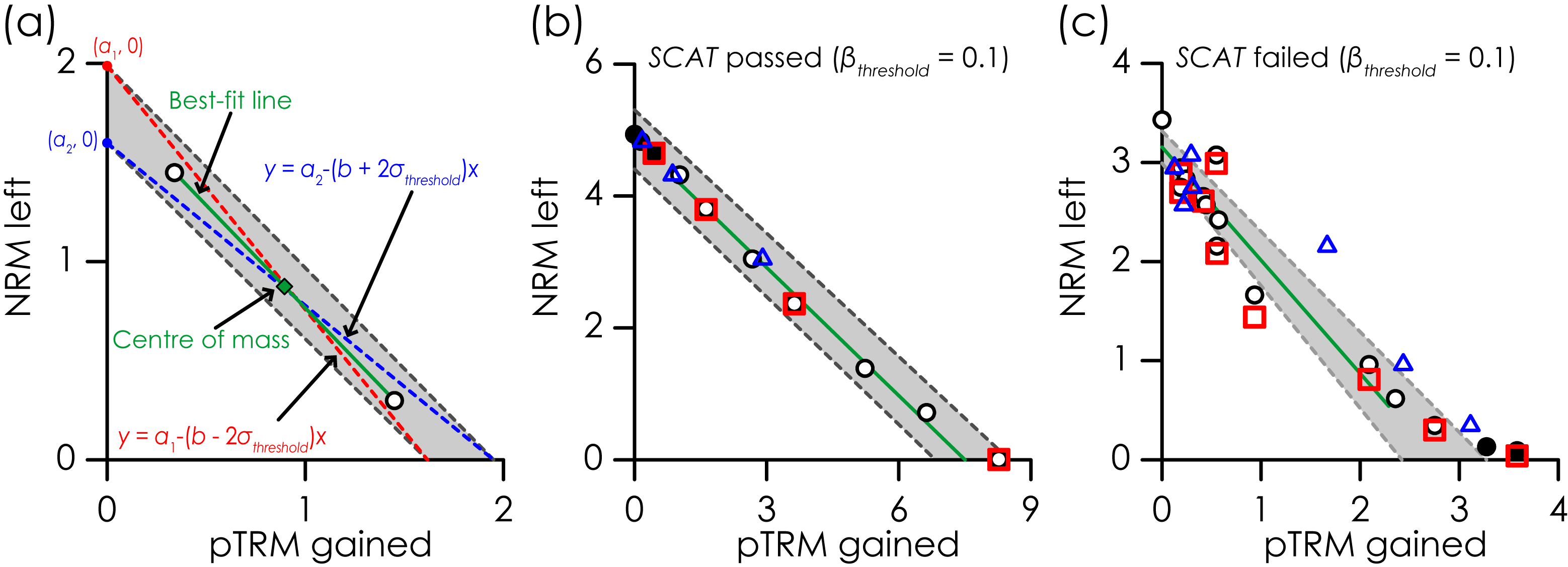
First, from the chosen the best-fit segment on the Arai plot, the slope (

$b$ ), the standard error of the slope (

$\sigma{}_b$ ), and

$\beta \left(=\frac{\sigma{}_b}{\left|b\right|}\right)$ are obtained. For a given sample, the threshold value for

$\beta$ that is used to select data (

$\beta{}_{threshold}$ ) is used to determine an equivalent threshold for

$\sigma{}_b$ (

$\sigma{}_{threshold}=\left|b\right|\beta{}_{threshold}$ ).

$b$ and

$\sigma{}_{threshold}$ are then used to determine two lines that pass through the center of mass of the selected Arai plot segment (

$\bar{x}$ and

$\bar{y}$ ), one with a slope of

$b+2\sigma{}_{threshold}$ , the other with a slope of

$b-2\sigma{}_{threshold}$ Figure 2a). The so called

$SCAT$ box, is the box that is defined by the four intercepts that the above two lines make with the x- and y-axes (Figure 2a).
If all the data points associated with the chosen Arai plot segment, which includes both pTRM and tail checks, fall within the

$SCAT$ box then

$SCAT$ is TRUE. If one or more points fall outside the

$SCAT$ box then

$SCAT$ is FALSE. Samples are accepted only if

$SCAT$ is TRUE. pTRM checks and pTRM tail checks are included in the calculation of

$SCAT$ if the temperature of the check falls within temperature range of the selected Arai plot segment and the peak temperature before the check was performed is less than or equal to maximum temperature of the selected Arai plot segment. For example, if the temperature range of the selected Arai plot segment was 100-500°C, a pTRM check to 200°C performed after the 400°C step would be included in the calculation of

$SCAT$ . However, a pTRM check to 200°C performed after the 540°C would be not included in the calculation of

$SCAT$ . Examples of samples pass and fail

$SCAT$ are shown in Figure 2b and c, respectively.

The correlation coefficient to estimate the strength of the linear relationship between the NRM and TRM over the best-fit Arai plot segment (the square of the Pearson correlation).

$R_{corr}^2=\frac{\left(\sum\limits_{i=start}^{end}(x_i-\bar{x})(y_i-\bar{y})\right)^2}{\sum\limits_{i=start}^{end}(x_i-\bar{x})^2\sum\limits_{i=start}^{end}(y_i-\bar{y})^2}$

Coefficient of determination to estimate variance accounted for by the linear model fit.

$R_{det}^2=1-\frac{\sum\limits_{i=start}^{end}{(y_i-y'_i)^2}}{\sum\limits_{i=start}^{end}{(y_i-\bar{y})^2}}$

Useful Note...
It should be noted that this is similar to, but strictly not the same as the square of the Pearson correlation coefficient ( $R_{corr}^2$ ). For least squares fitting that minimizes the y residuals only, $R_{corr}^2$ is the same as the coefficient of determination for the model fit. Since Arai plot analysis uses the standardized major axis least-squares variant, this is not the case. For most practical purposes, however, the difference is small, particularly when the chosen Arai plot segment is highly linear with low noise.

$Z$ is an Arai plot zigzag parameter defined by Yu and Tauxe (2005).

$Z=\sum\limits_{i=start}^{end}{\frac{x_i\left|\tilde{b}_i-\left|b\right|\right|}{\left|X_{Int.}\right|}},$ where

$\tilde{b}_i$ is the instantaneous slope on the Arai plot determined from the ratio of the NRM lost to the TRM gained at the

$i^{th}$ step:

$\tilde{b}_i=\frac{NRM_{total} - NRM_i}{TRM_i}=\frac{Y_{Int.} - y_i}{x_i}.$ Since no TRM is gained during the first step

$\tilde{b}_1=0$ .

$\tilde{b}_i-\left|b\right|$ is a measure of the scatter around the best-fit slope on the Arai plot.

Yu (2012) proposed a modified version,

$Z^*$ .

$Z^*=\frac{1}{n-1}\sum\limits_{i=start}^{end}{100\times\frac{x_i\left|\tilde{b}_i-\left|b\right|\right|}{\left|Y_{Int.}\right|}}.$

$IZZI\_MD$ is a parameter to quantify the zigzagging on an Arai plot (Shaar et al., 2011), which is most pronounced for multidomain grains measured with the IZZI protocol (e.g., Yu et al., 2004).

$IZZI\_MD$ is a measure of the area mapped out on the Arai plot and is determined using all the points on an Arai plot with the exception of the first step, where no TRM is imparted. The calculation is performed after the points have been normalized by the initial NRM, such that

$x_{(n)i}=\frac{x_i}{y_1}~~\textrm{and}~~y_{(n)i}=\frac{y_i}{y_1}.$

If we consider the three consecutive Arai plot points illustrated in Figure 3a. The lengths of each side of the triangle formed by these points are given by:

$L_1=\sqrt{\left(x_{(n)i}-x_{(n)i+1}\right)^2 + \left(y_{(n)i}-y_{(n)i+1)}\right)^2};$

$L_2=\sqrt{\left(x_{(n)i+1}-x_{(n)i+2}\right)^2 + \left(y_{(n)i+1}-y_{(n)i+2}\right)^2};$ and

$L_3=\sqrt{\left(x_{(n)i+2}-x_{(n)i}\right)^2 + \left(y_{(n)i+2}-y_{(n)i}\right)^2}.$

Following the cosine rule, the angle

$\phi$ is

$\phi=\arccos\left(\frac{L_2^2+L_3^2-L_1^2}{2L_2L_3}\right).$ The height of the triangle can be expressed as

$H=L_3\sin\left(\phi\right),$ and hence the area of the triangle is given by

$A_i=\frac{L_2L_3\sin\left(\phi\right)}{2}.$

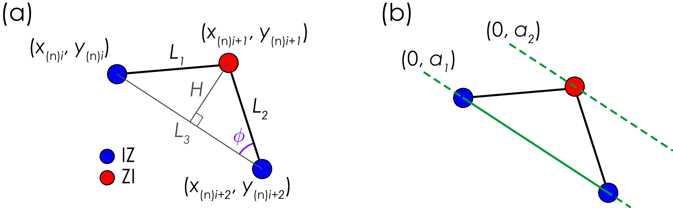
Each

$A_i$ is given a sign (

$\pm$ ) based on whether or not the ZI steps lie above the IZ steps, or vice versa. For ZI above IZ,

$A_i$ is positive, for IZ above ZI,

$A_i$ is negative. For the example in Figure 3, ZI is above IZ and the area is given a positive sign.
To determine the sign, we must determine the relative position of the mid-point of the three consecutive points. First, we calculate the best-fit line through the first and last points and obtain the intercept of the line (

$a_1$ ; Figure 3b). Using the slope of this best-fit line we determine the intercept of the line (

$a_2$ ) when the line passes through the mid-point. If

$a_1$ is less than

$a_2$ the mid-point lies above the end points, but if

$a_2$ is less than

$a_1$ the mid-point lies below the end points. In the case where

$a_1=a_2$ all three points lie on a perfect straight line and both the area and the sign are identically zero. The pseudo-code for this is as follows, where

$S_i$ denotes the sign of the

$i^{th}$ area.

for $i = 2 \rightarrow (n_{max}-2)$ do
    if $a_1 = a_2$ then
         $S_i=0$
    else
        if Mid-point is a ZI then
            if $a_1 < a_2$ then
                 $S_i=1$           ←{Figure 3b falls here}
            else
                 $S_i=-1$
            end if
        else if Mid-point is a IZ then
            if $a_1 < a_2$ then
                 $S_i=-1$
            else
                 $S_i=1$
            end if
        end if
    end if
end for

$IZZI\_MD$ is the sum of the signed areas, normalized by length of the line connecting all of the ZI steps.

$IZZI\_MD=\sum\limits_{i=2}^{n_{max}-2}\frac{S_iA_i}{L_{ZI}}.$ where

$L_{ZI}$ is given by:

$L_{ZI}=\sum\limits_{i \in~ZI~points}^{}\sqrt{\left(x_{(n)i+2}-x_{(n)i}\right)^2 + \left(y_{(n)i+2}- y_{(n)i}\right)^2}~.$
N.B. The

$i+2$ increment assumes alternating ZI and IZ step, whereby if

$i$ is a ZI step,

$i+1$ is an IZ step, and

$i+2$ is a ZI step.

Numerical Tip...
Calculating the area bounded by a series of points is a common geometric problem. As a consequence most programming languages have functions to perform the calculation either as inbuilt features or as freely available routines. For example, MATLAB has the inbuilt function A=polyarea(p) to return the area, A , bounded by the points given by the two-dimensional matrix p : $\mathbf{p}= \begin{pmatrix} x_{i} & y_{i} \\ x_{i+1} & y_{i+1} \\ x_{i+2} & y_{i+2} \\ \end{pmatrix}$

3 Arai plot statistics

3.1 A note on data indexing

3.2 The paleointensity estimate

3.3 Arai plot statistics