Home          Downloads          SPD on the web          Links

[← Arai plot statistics]     [↑ SPD on the web]      [pTRM check statistics →]

4 Directional statistics

Statistic: $$Dec$$ and $$Inc$$
Report to 1 d.p.

The declination ($$Dec$$) and the inclination ($$Inc$$) of NRM direction of the paleointensity data over the same range of points used for the paleointensity estimates. $$Dec$$ and $$Inc$$ are calculated using the principal component analysis (PCA) method of Kirschvink (1980) and may be obtained from either a free-floating or anchored fit.

The method of applying PCA to paleomagnetic data is as follows. Let $$X_{1,i}$$, $$X_{2,i}$$, and $$X_{3,i}$$ denote the $$x$$, $$y$$, and $$z$$ Cartesian coordinates of the NRM vector of the selected points ($$i=start\ldots end$$). The center of mass of the data is given by the ordinates $$\bar{X_{1}}$$, $$\bar{X_{2}}$$, and $$\bar{X_{3}}$$. \[ \bar{X_{1}}=\frac{\sum\limits_{i=start}^{end}{X_{1,i}}}{n};~~~\bar{X_{2}}=\frac{\sum\limits_{i=start}^{end}{X_{2,i}}}{n};~~~ \bar{X_{3}}=\frac{\sum\limits_{i=start}^{end}{X_{3,i}}}{n} \]

The coordinates of the NRM vector are then transformed to be centered about $$\bar{X_{1}}$$, $$\bar{X_{2}}$$, and $$\bar{X_{3}}$$. \[ X'_{1,i}=X_{1,i} - \bar{X_{1}};~~~X'_{2,i}=X_{2,i} - \bar{X_{2}};~~~ X'_{3,i}=X_{3,i} - \bar{X_{3}}, \] where $$X'_{1,i}$$, $$X'_{2,i}$$, and $$X'_{3,i}$$ are the transformed coordinates. A fit anchored to the origin of the component diagram can be obtained by setting [$$\bar{X_{1}}$$, $$\bar{X_{2}}$$, $$\bar{X_{3}}$$] to [0, 0, 0].

The orientation tensor, $$\mathbf{T}$$, of the transformed NRM data is defined as: \[ \mathbf{T}= \begin{pmatrix} \sum{X'_{1,i}X'_{1,i}} & \sum{X'_{1,i}X'_{2,i}} & \sum{X'_{1,i}X'_{3,i}} \\ \sum{X'_{1,i}X'_{2,i}} & \sum{X'_{2,i}X'_{2,i}} & \sum{X'_{2,i}X'_{3,i}} \\ \sum{X'_{1,i}X'_{3,i}} & \sum{X'_{2,i}X'_{3,i}} & \sum{X'_{3,i}X'_{3,i}} \\ \end{pmatrix}. \] This orientation tensor is usually constructed within sample or geographic coordinates and consists of six independent elements. Typically, none of these elements zero. When the non-diagonal elements of $$\mathbf{T}$$ are non-zero the vector components described by this coordinate system are not independent, they are correlated. There exists, however, a coordinate system in which the orientation tensor can be expressed in terms of three independent orthogonal components. The axes of this coordinates system are known as the eigenvectors of the matrix and can be expressed in linear algebra form as: \[ \mathbf{TV}=\tau\mathbf{V}, \] where $$\mathbf{V}$$ is a matrix that contains the three eigenvectors (also know as principal axes) and $$\tau$$ is a diagonal matrix that contains the three eigenvalues. When ranked by $$\tau$$, such that $$\tau{_3} < \tau{_2} < \tau{_1}$$, the principal axis (i.e., $$\mathbf{V}_1=\left[V_{1,x}, V_{1,y}, V_{1,z}\right]$$) corresponds to axis of the characteristic paleomagnetic direction.

It should be noted, however, that paleomagnetic direction may be either parallel or anti-parallel to $$\mathbf{V}_1$$ and the sense of direction must be established. To do this, we define a reference vector ($$\mathbf{R}$$) defined as the difference between the first and last NRM vector measurements: \[ \mathbf{R}=\mathbf{X'}_{i=start}-\mathbf{X'}_{i=end}=\left[X'_{1,start}-X'_{1,end}, X'_{2,start}-X'_{2,end}, X'_{3,start}-X'_{3,end}\right]. \]

The vector dot product of $$\mathbf{V}_1$$ and $$\mathbf{R}$$ is then determined. \[ dot=\mathbf{V}_1\cdot{}\mathbf{R} = V_{1,x}\times{}R_{x} + V_{1,y}\times{}R_{y} + V_{1,z}\times{}R_{z} \]

The range of $$dot$$ is then truncated to exist only over [-1, 1].

The principal paleomagnetic direction ($$\mathbf{PD}=\left[PD_x, PD_y, PD_z\right]$$ can be given a sense of direction along $$\mathbf{V}_1$$ as follows.

The declination ($$Dec$$) and inclination ($$Inc$$) of principal paleomagnetic direction can be calculated.

Statistic: $$MAD_{Anc.}$$ and $$MAD_{Free}$$
Report to 1 d.p.

$$MAD_{Anc.}$$ and $$MAD_{Free}$$ are Maximum Angular Deviation (MAD) of the anchored and free-floating, respectively, directional fits to the paleomagnetic vector on a vector component diagram (Kirschvink, 1980). Determined from the paleointensity demagnetization steps.

$$MAD$$ is calculated as: \[ MAD=\arctan{ \left( \sqrt{ \frac{ \tau{_{2}}+\tau{_{3}} }{\tau{_{1}}} }\right) }, \] where $$\tau{_{3}} < \tau{_{2}} < \tau{_{1}}$$ are the eigenvalues of the PCA matrix.

Statistic: $$\alpha$$
Report to 1 d.p.

Angular difference between the anchored and free-floating best-fit directions on a vector component diagram.

Statistic: $$\alpha'$$
Report to 1 d.p.

Angular difference between the anchored best-fit direction from the paleointensity experiment and an independent measure of the paleomagnetic direction (Kissel and Laj, 2004). The independent direction can be derived from a separate demagnetization experiment or from a known reference direction.

Statistic: $$\theta$$
Report to 1 d.p.

The angle between the applied field direction and the ChRM direction of the NRM as determined from the free-floating PCA fit to the selected demagnetization steps of the paleointensity experiment.

Statistic: $$DANG$$
Report to 1 d.p.

The Deviation ANGle: the angle between the free-floating best-fit direction and the direction between data center of mass [$$\bar{X_{1}}, \bar{X_{2}}, \bar{X_{3}}$$] and the origin of the vector component diagram (Tanaka and Kobayashi, 2003; Tauxe and Staudigel, 2004).

Statistic: $$NRM_{dev}$$
Report to 1 d.p.

The intensity deviation of the free-floating principal component from the origin of the vector component diagram, normalized by the total NRM intensity ($$Y_{Int.}$$; Tanaka and Kobayashi, 2003). \[ NRM_{dev}=\frac{\sin{(DANG)}\sqrt{\bar{X_{1}}^2 + \bar{X_{2}}^2 + \bar{X_{3}}^2}}{\left|Y_{Int.}\right|}\times{100} \]

Statistic: $$\gamma$$
Report to 1 d.p.

The angle between the pTRM acquired at the last step used for the best-fit segment (i.e., $$\mathbf{TRM}_{i=end}$$) and the applied field direction ($$\mathbf{B}_{Lab}$$). $$\gamma$$ can be used as a quick check to assess if a sample is strongly influenced by anisotropic TRM. See Section 8 for further information of measuring and quantifying anisotropy of TRM.

Statistic: $$CRM(\%)$$
Report to 1 d.p.

To detect the potential acquisition of chemical remanent magnetization (CRM), Coe et al. (1984) proposed $$CRM(\%)$$ to measure the deflection the NRM vector towards the direction of $$B_{Lab}$$ as would be expected during the formation of CRM. A schematic illustration of the quantities involved in the calculation of $$CRM(\%)$$ are shown in Figure 4. To determine $$CRM(\%)$$ the characteristic remanent magnetization (ChRM) direction needs to be known. This must be determined from an independent demagnetization experiment.

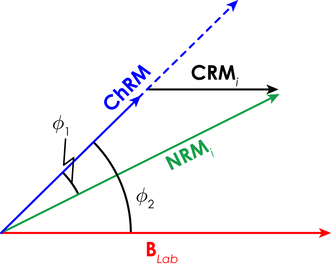
First, the magnitude of the CRM vector is determined: \[ CRM_i=\left\|\mathbf{NRM}_i\right\|\frac{\sin{(\phi_1)}}{\sin{(\phi_2)}}=y_i\frac{\sin{(\phi_1)}}{\sin{(\phi_2)}}, \] where $$\left\|\mathbf{NRM}_i\right\|$$ denotes the length of the $$\mathbf{NRM}_i$$ vector, which is equivalent to $$y_i$$.

$$CRM(\%)$$ is the maximum value of $$CRM_i$$ over the selected best-fit Arai segment, normalized by the length of the TRM portion of best-fit Arai line: \[ CRM(\%)=\frac{\max{\left\{CRM_i\right\}}_{i=start, \ldots, end}}{\Delta{x'}}\times{100}. \]